Modelling the imaging system

Modelling the imaging system can be rather complex due to many small something something and technicalities. The light hitting the sensor is dependent on both the wavelength as well as the mirror separation of the scanning Fabry-Pérot interferometer (SFPI). Furthermore, the position on the sensor also has an effect on the spectral profile. That is because the incidence angle increases as we move away from the center of the frame. A larger angle of incidence mean that shorter wavelengths are transmitted compared to normal incidence. The worst case is 17.25 º which results in 95.5 % shorter wavelengths compared to the middle. We are going to ignore this effect in this post in an attempt to reduce the complexity just a bit.

Processing and how to interpret the data

Another challenge is how to interpret the data and what we are “allowed” to do during data processing. Each frame of the data cube represent the distribution of light coming through the SFPI at a given mirror separation - and then we need to account for the sensor response as well (which is really the combined response of the sensor and the transmission of the germanium optics in front of it). A single frame is a 16-bit image, but only storing 14 bits of information. That means that the raw signal consists of integers ranging from 0 to 65535 with a resolution of 4 (minimal difference between two values). It is however often, that it is difficult to see, what is in a frame based on the raw image because of the non-uniformity of the sensor. Pixels are not made equally, and that is especially the case for a microbolometer. At the same light intensity, two pixels may produce vastly different outputs (some may be entirely dead, even). The responsivity (change of output per change of input) is also different across pixels. In “regular” thermal cameras, this is counteracted by applying a non-uniformity correction (NUC) to the image (Fig. 1). This correction shifts the value of each pixel in the image to equalize the variations in the image based on previous calibrations, which are both dependent on the sensor temperature and the GSK voltage. The GSK voltage is a camera setting used to apply an offset to the pixels, which ensures that all (or at least most) of the values lies within the linear range of the sensor. The NUC is not perfect and especially when working with rather low signals as in the case of the hyperspectral camera, some residual noise is still left in the image. However, one of the advantages of this post processing step is that the pixel values remain roughly the same (the mean of the image stays about the same).

Figure 1: a) Raw image out of the data cube. b) Same image as in a) but after non-uniformity correction.

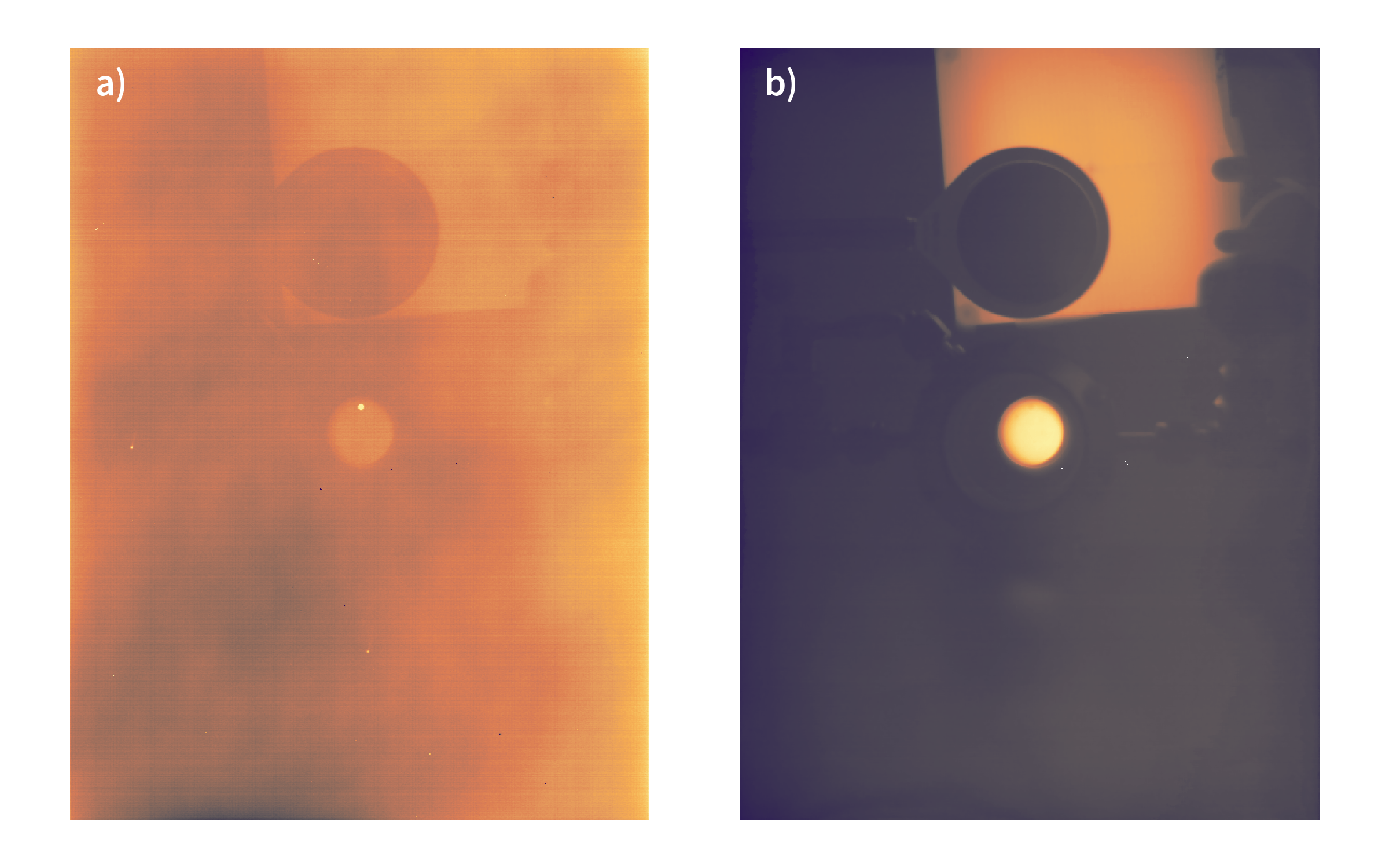
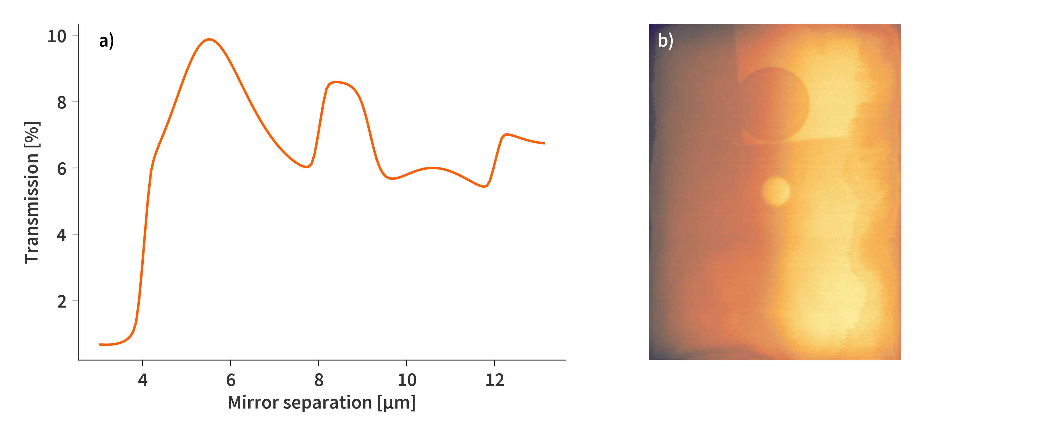
In some instances, it is not possible to perform the NUC because the sensor temperature is outside the temperature range at which it has been calibrated (17 ºC to 30 ºC). Here, it is convenient to use the first image of the data cube as a form of “dark frame” as almost no light (at least within the sensitive range of the sensor) is let through the SFPI at this mirror separation. The first image is then subtracted from all layers of the cube, effectively setting the first layer to $\mathbf{0}$. However, the assumption of “No light is getting through” is not quite correct. If we ignore the sensitivity of the sensor and purely focus on the transmission of the SFPI calculated using the Transfer Matrix Method (TMM) in the range from from ≈ 1250 cm^-1 ($\lambda = 8$ µm) to ≈ 650 cm^-1 ($\lambda = 15.38$ µm), the transmission is at most 9.9 % at a single frame. Above mirror separations of 5 µm, the average is about 7 %. So generally not much light to collect in the first place. When the mirrors are completely together, there is still 0.7 % of the light getting through and onto the sensor. It does not sound like much, but this is still about 7% of the signal at maximum transmission. Performing NUC on the first image of the data cube (when the mirrors are completely closes) reveal that there is still plenty of information to extract (Fig. 2). However, the residual errors from the NUC are now much more noticeable due to the smaller signal fluctuations across the frame.

Figure 2: a) Light transmission compared to if there was no SFPI b) First image of the data cube corrected using NUC.

Why not always use the NUC if the sensor temperature is within range?

Good question - I would also prefer this, but there are some caveats. Firstly, the output is very sensitive to the sensor temperature. The resolution of the sensor temperature measurements is ≈ 0.3 ºC, which is still quite a lot in terms of the signal output. Secondly, the temperature of the environment and the lens housing might also affect the images significantly (enough to be detectable at least). During the measurement series, the temperature of the laboratory is subject to change and the lens temperature was not monitored. However, subsequent testing indicate that the temperature of the lens housing is rather constant at around 25 ºC over the span of a weekend (read more here).

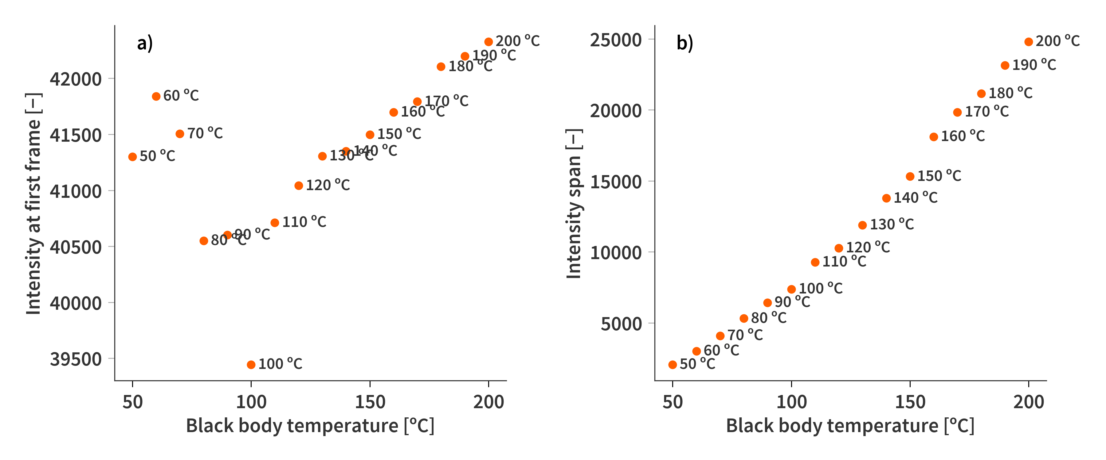
In the data series acquired to solve the inverse problem (and fit sensor response), there is i.a. a series of black body measurements at varying temperatures. The first frame of each of the images do in fact follow a linear trend as expected with the exception of a couple of measurements, which are a bit all over the place (Fig. 3). However, if we look at the span (difference between minimum and maximum value of the interferogram) the same measurements fall back in line. So this means that the entire data cube is offset - possibly by wrong temperature readings or maybe by changing temperatures of the lens housing… The NUC could also be imperfect (well it is), but the results are similar if I use the images completely unprocessed… I dunno, but these discrepancies make it really difficult to train a model to correlate the raw intensity output to an absolute exitance. For this reason, the most common processing step is to subtract the first frame of the data cube, but that introduces some other caveats. For example that parts of the interferogram can become negative as it is possible to have more light leaving the system than is entering it. This is not an expression of “negative light”, but rather a consequence of where the zero-point has been set by using the first frame as a reference. Furthermore, the signal from the microbolometer sensor is proportional to the difference in flux - not the absolute flux hitting the sensor. This might give some interesting implications when trying to model the system later, since negative contributions does not really make much physical sense and might not play well with the solvers/methods, which sometimes require non-negativity in all parts of the model.

Figure 3: a) The intensity of the black body interferograms at the first image of the cubes. b) The span (difference between maximum and minimum value) of the interferograms for each of the black body measurements.

Modelling the system

As with any good $\mathbf{Ax}=\mathbf{b}$ problem, the system can be described in three parts. However, there are a few permutations which can be made to describe the same system and they each have their advantages and disadvantages. Usually, the matrix $\mathbf{A}$ is some variation of the system matrix describing the relationship between transmission of the SFPI, its mirror separation and the wavelength of the incident light. In that case, $\mathbf{x}$ is the incident spectrum and $\mathbf{b}$ is the recorded interferogram (spectral axis of the data cube).

Now, lets start by defining the flux incident on the sensor

\[\begin{align} \label{eq:fpi_flux} \mathbf{\Phi_{in}} = \mathbf{T_{SFPI}}\diamond[\mathbf{t_{samp}}\circ\mathbf{m_{BB}}(T_{BB}) + \mathbf{r_{samp}}\circ\mathbf{m_{env}}(T_{env})] + \mathbf{R_{SFPI}} \diamond \mathbf{m_{sens}}(T_{sens}) \end{align}\]

Here, $\diamond$ and $\circ$ refer to element wise and row wise multiplication respectively. $\mathbf{T_{SFPI}}$ and $\mathbf{R_{SFPI}}$ are matrices describing the transmittance and reflectance of the SFPI respectively. Each row of the matrices is denoted to a specific mirror separation, with each column ascribed to a specific wavelength/wavenumber. $T_{BB}$, $T_{env}$, and $T_{sens}$ are the temperatures of the black body behind the sample and the temperature of the environment. $\mathbf{m}$ is a vector describing the black-body emission spectrum where the subscripts refer to the source of radiation (black-body, environment, and sensor). $\mathbf{t_{samp}}$ and $\mathbf{r_{samp}}$ are the transmission and reflectance spectrum of the sample respectively. The length of the vectors are the same as the number of columns in $\mathbf{T_{SFPI}}$ and $\mathbf{R_{SFPI}}$.

An argument could be made for also including a flux term from the sensor housing, objective, lenses and SFPI itself as they also have a temperature, which is most often different from the sensor temperature. A good estimate would probably be to approximate this term by another $\mathbf{m_{env}}(T_{env})$ or ideally by knowing the temperature inside the lens itself, but it has initially been left out.

What we want to solve for in the end is

\[\begin{align} \label{eq:x} \mathbf{x} = \mathbf{t_{samp}}\circ\mathbf{m_{BB}}(T_{BB}) + \mathbf{r_{samp}}\circ\mathbf{m_{env}}(T_{env}) \end{align}\]

which is the spectrum of the light entering the camera.

The signal recorded by the camera is however not directly proportional to the incident flux. Rather, the signal is proportional to the difference in flux between the sensor and the incident radiation. That is

\[\begin{align} \label{eq:signal} \mathbf{i} \propto [\mathbf{\Phi_{in}} - \mathbf{m_{sens}}(T_{sens})]\mathbf{s} \end{align}\]

Here, $\mathbf{i}$ represent the interferogram that is recorded while moving the mirrors of the SFPI. The length of $\mathbf{i}$ is the same as the number of rows in $\mathbf{T_{SFPI}}$. The difference in flux is expressed by $[\mathbf{\Phi_{in}} - \mathbf{m_{sens}}(T_{sens})]$. Again the subtraction is done row-wise. $\mathbf{s}$ is the spectral response of the sensor (same number of elements as columns in $\mathbf{T_{SFPI}}$).

Modelling system matrix

Strictly speaking, $\mathbf{T_{SFPI}}$ is just the transmission matrix of the SFPI at different mirror separations and wavelengths. The system matrix would also include the spectral sensitivity of the sensor as well as the transmission spectrum of the germanium optics between the SFPI and the sensor. We already have quite a good understanding of $\mathbf{T_{SFPI}}$ which is calculated based on TMM (or GMM to be exact) and presented in Fig 4.

Figure 4: a) Transmission matrix of SFPI calculated from TMM. Broadening simulating mirror bending of 150 nm has been applied. b) is the same transmission matrix as in a), but with the sensor response applied

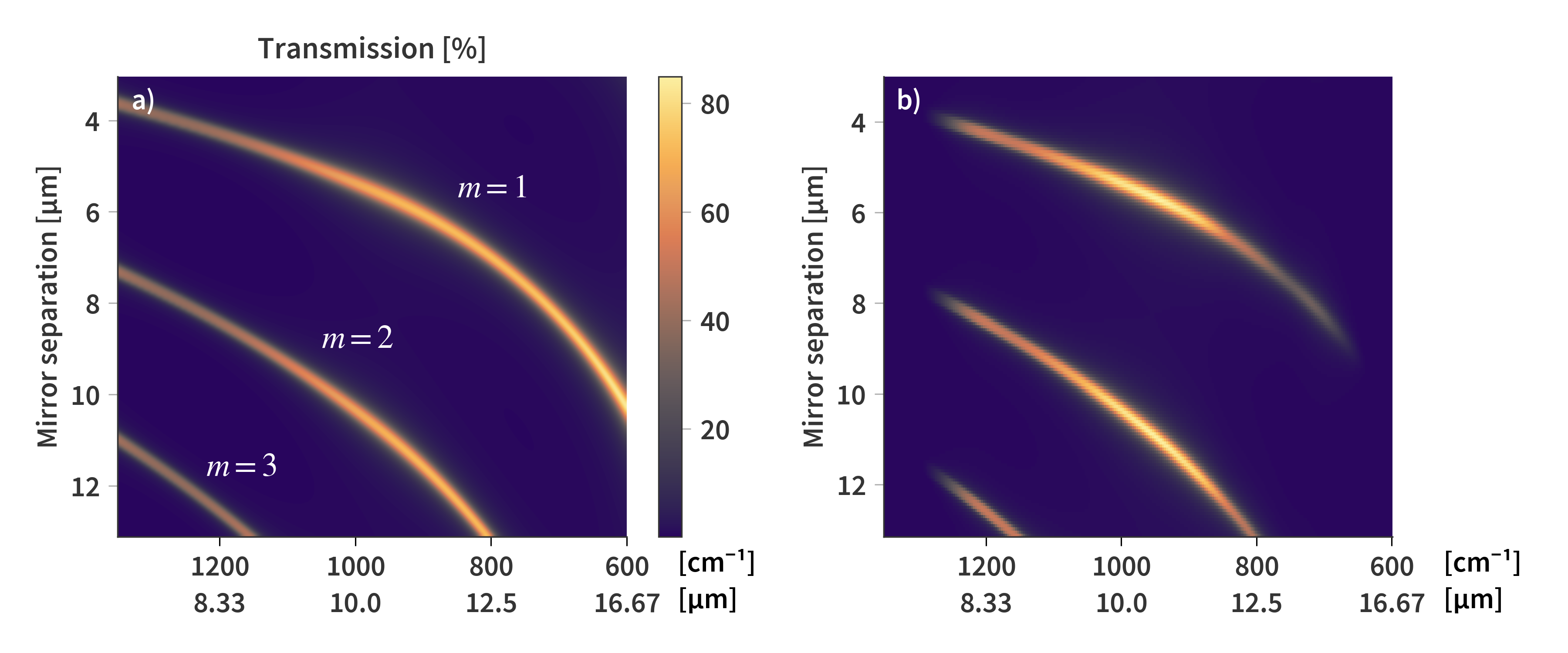
This representation is only mostly correct and absorptive losses have not been taken into account. It would be nice to use this as a starting point for the system matrix where the response of the sensor and optics are also accounted for. I would expect for the true solution to have the same overall structure, but the heights and widths of the transmission orders as well as their location might deviate slightly, but should still be smooth in either direction as well as lie between 0 and 1.

Ax=b Configuration 1

The first way to rearrange the terms into an $\mathbf{Ax}=\mathbf{b}$ problem is by embedding the sensor response directly in the transmission matrix. That way we can write the system matrix as

\[\begin{align} \label{eq:sys_matrix_1} \mathbf{A} = \mathbf{T_{SFPI}}\diamond\mathbf{s} \end{align}\]

The other terms not part of $\mathbf{x}$ is moved to the left-hand side of Eq. (\ref{eq:signal}).

\[\begin{align} \label{eq:Ax=b1} \mathbf{i} - [(\mathbf{R_{SFPI}} - \mathbf{1}) \diamond \mathbf{m_{sens}}(T_{sens})]\mathbf{s} + \psi = \mathbf{Ax} \end{align}\]

In this variation there are no negative terms in neither $\mathbf{A}$ nor $\mathbf{x}$ as it is moved to $\mathbf{b}$ instead. Note that $[(\mathbf{R_{SFPI}} - \mathbf{1}) \diamond \mathbf{m_{sens}}(T_{sens})]\mathbf{s}$ is exclusively negative since $\mathbf{R_{SFPI}}$ cannot be greater than 1. This way $\mathbf{A}$, $\mathbf{x}$, and $\mathbf{b}$ are all exclusively nonnegative. $\psi$ represents an offset to the entire interferogram. That could be the offset introduced by the GSK-voltage or in the data processing. The important thing is that it is a constant offset across all measurements (no spectral dependence) and can be either negative, zero, or positive.

Here, we want to solve for $\mathbf{x}$ which is the input spectrum and we know everything else, except $\psi$. The final cost function can then be expressed as:

\[\begin{align} \label{eq:arg_min1} &\arg \min_{\mathbf{x}, \: \psi} ||\mathbf{b} + \psi - \mathbf{Ax}||_2^2 + \gamma||\mathbf{Mx}||_2^2 , \quad \textrm{s.t.} \quad \mathbf{x} \geq 0 \\[1.2em] &\mathbf{b} = \mathbf{i} - [(\mathbf{R_{SFPI}} - \mathbf{1}) \diamond \mathbf{m_{sens}}(T_{sens})]\mathbf{s} \end{align}\]

where $\gamma||\mathbf{Mx}||_F^2$ is a regularization term promoting a smooth solution.

Ax=b Configuration 2

Here, we are going to work with the same system matrix as before, namely $\mathbf{A} = \mathbf{T_{SFPI}}\diamond\mathbf{s}$. Additionally, it is assumed that the SFPI is lossless meaning $\mathbf{R_{SFPI}} = \mathbf{1} - \mathbf{T_{SFPI}}$. Eq. (\ref{eq:fpi_flux}) then becomes

\[\begin{align} \label{eq:fpi_flux2} \mathbf{\Phi_{in}} &= \mathbf{T_{SFPI}}\diamond[\mathbf{t_{samp}}\circ\mathbf{m_{BB}}(T_{BB}) + \mathbf{r_{samp}}\circ\mathbf{m_{env}}(T_{env})] + (\mathbf{1} - \mathbf{T_{SFPI}}) \diamond \mathbf{m_{sens}}(T_{sens}) \\[1.2em] &= \mathbf{T_{SFPI}}\diamond[\mathbf{x} - \mathbf{m_{sens}}(T_{sens})] + \mathbf{m_{sens}}(T_{sens}) \end{align}\]

Eq. (\ref{eq:signal}) then becomes

\[\begin{align} \label{eq:signal2} \mathbf{i} \propto (\mathbf{T_{SFPI}}\diamond[\mathbf{x} - \mathbf{m_{sens}}(T_{sens})])\mathbf{s} = \mathbf{A}[\mathbf{x} - \mathbf{m_{sens}}(T_{sens})] = \mathbf{A}\mathbf{\chi} \end{align}\]

We know (or at least are able to estimate $\mathbf{m_{sens}}(T_{sens})$) which means that if we find $\mathbf{\chi}$, we can calculate $\mathbf{x}$ by subtracting $\mathbf{m_{sens}}(T_{sens})$. The final $\mathbf{Ax}=\mathbf{b}$ then becomes:

\[\begin{align} \label{eq:Ax=b2} \mathbf{i} + \psi = \mathbf{A\chi} \end{align}\]

In this case, the negative terms are moved to $\mathbf{\chi}$ instead, making $\mathbf{i}$ and $\mathbf{A}$ purely nonnegative while $[\mathbf{x} - \mathbf{m_{sens}}(T_{sens})]$ can actually be negative if the net flux becomes negative. Again, $\psi$ is included to represent the interferogram offset.

The cost function for this variation of the minimization problem then becomes:

\[\begin{align} \label{eq:arg_min2} &\arg \min_{\mathbf{\chi}, \: \psi} ||\mathbf{i} + \psi - \mathbf{A\chi}||_2^2 + \gamma||\mathbf{M\chi}||_2^2 \end{align}\]

Dictionary of Gaussians

There is a limit to how fine details can be resolved using the SFPI. We’re going to use the criterion that two adjacent features should be at least on Full Width at Half Maximum (FWHM) apart to be resolvable. For this discussion we’re going to start by looking at the theoretical expression for the transmission through the SFPI described by the Airy function

\[\begin{align} \label{eq:airy} T = \frac{1}{1 + 4\mathcal{F}^2/\pi^2 \sin^2{\delta}}, \qquad \delta = 2\pi\tilde{\nu}d \qquad \tilde{\nu} = \frac{1}{\lambda}, \qquad \mathcal{F} = \frac{\pi r}{1-r^2}, \end{align}\]

where $\tilde{\nu}$ is the wavenumber, $\lambda$ the wavelength, $d$ is the mirror separation, $\mathcal{F}$ is the finesse of the SFPI, and $r$ is the mirror reflectance.

Eq. (\ref{eq:airy}) reaches a maximum whenever the phase $\delta = m\pi, \quad m = 1, 2, 3, \dots$. That meas the distance between two neighboring maxima (Free spectral range - FSR) can be expressed as

\[\begin{align} \label{eq:fsr} \delta_\textrm{fsr} = \delta_{m+1} - \delta_{m} = (m+1)\pi - m\pi = \pi \end{align}\]

Using Eq. (\ref{eq:fsr}) we can express the FSR both in terms of wavenumbers and in terms of mirror separation as

\[\begin{align} \label{eq:fsrs} &2\pi\tilde{\nu}_\textrm{fsr}d = \pi \\[1.1em] \Rightarrow & \tilde{\nu}_\textrm{fsr} = \frac{1}{2d} \label{eq:k_fsr}\\[1.1em] \Rightarrow & d_\textrm{fsr} = \frac{1}{2\tilde{\nu}} \label{eq:d_fsr} \end{align}\]

Just as an aside (and mostly for my own reference), the FSR in terms of wavelength can be calculated by

\[\begin{align} \label{eq:wavl_fsr} &\lambda_\textrm{fsr} = \lambda_{m+1} - \lambda_{m} = \frac{2d}{m+1} -\frac{2d}{m} = \frac{2d}{2d/\lambda+1} -\frac{2d}{2d/\lambda} \nonumber\\[1.1em] \Rightarrow& (\lambda_\textrm{fsr} + \lambda)\left(\frac{2d}{\lambda} + 1\right)= 2d \nonumber\\[1.1em] \Rightarrow& \frac{2d\lambda_\textrm{fsr}}{\lambda} + \lambda_\textrm{fsr} + \lambda = 0 \nonumber\\[1.1em] \Rightarrow& \lambda_\textrm{fsr} = \frac{\lambda}{2d/\lambda +1} = \frac{\lambda^2}{2d+\lambda} \\[1.1em] \end{align}\]

The FSR can be used to calculate the FWHM of the SFPI at a given combination of wavelength and mirror separation based on the finesse which can also be expressed as:

\[\begin{align} \label{eq:finesse} \mathcal{F} = \frac{\delta_\textrm{fsr}}{\delta_\textrm{FWHM}} = \frac{\tilde{\nu}_\textrm{fsr}}{\tilde{\nu}_\textrm{FWHM}} \end{align}\]

Solving for the FWHM in terms of wavenumbers gives us

\[\begin{align} \label{eq:nu_FWHM} &\tilde{\nu}_\textrm{FWHM} = \frac{\tilde{\nu}_\textrm{fsr}}{\mathcal{F}} = \frac{1}{2\mathcal{F}d}\\ &\lambda_\textrm{FWHM} = \frac{\lambda^2}{2\mathcal{F}d} \qquad \textrm{(From Pedrotti)} \end{align}\]

This means that the FWHM is not frequency dependent but does depend on wavelength. In both cases it does decrease (higher resolving power) at longer mirror separations. Only the first transmission order covers all wavelengths with the limited range of the SFPI (mirror separations from 3 $-$ 13 µm). The two higher orders which can be observed only cover the shorter wavelengths which is why these are better resolved. To find the theoretical best (smallest) FWHM, one could just use Eq. (\ref{eq:nu_FWHM}) and set the mirror separation to the highest possible - in this case ≈ 13 µm - but only a small subsection of wavelengths are transmitted at this mirror separation. Based on the system matrix in Fig. 4b, only combinations of mirror separations and wavelengths where the sensitivity is above 5 % of the maximum value is considered for the FWHM calculations. This is why there are discontinuities in the depiction of the FWHM in Fig. 5. The shorter wavelengths utilize the third order and hereby better FWHM, while the longest wavelengths can only use the first transmission order.

Figure 5: a) Finesse of the SFPI calculated based on Eq. (\ref{eq:finesse}) and reflection FTIR measurements of the mirrors. b) Full Width at Half Maximum of the SFPI throughout the spectral range.

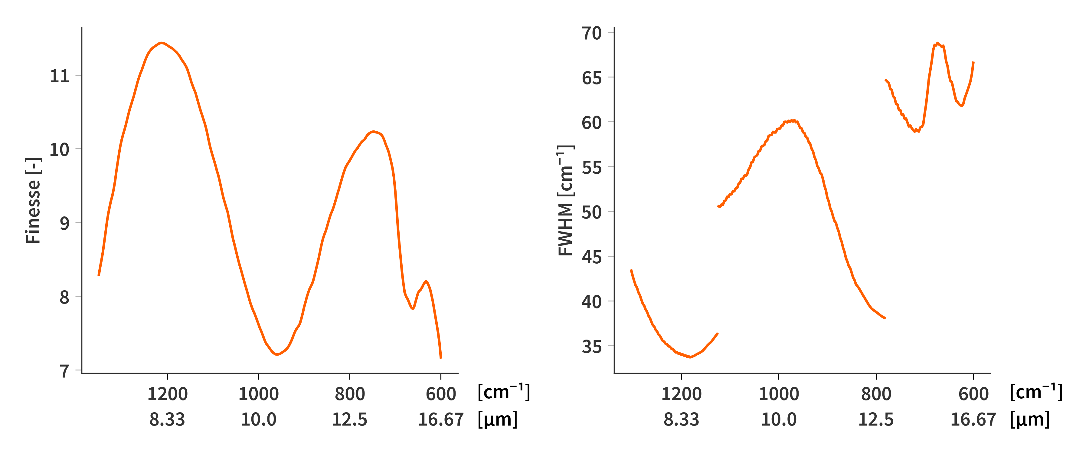
Next is just to make a dictionary of Gaussians with the FWHM as predicted in Fig. 5.

Since only wavelengths above 5 % are considered, there are some wavelengths which is not associated with a peak width. The spectral range of the system (this also goes for the system matrix in Fig. 4b) has therefore been truncated to only span from 1276 cm^-1 ($\lambda = 7.8$ µm) to ≈ 658 cm^-1 ($\lambda = 15.2$ µm) _{compared to the original 1300 cm^-1 ($\lambda = 7.4$ µm) to ≈ 600 cm^-1 ($\lambda = 16.7$ µm)} .

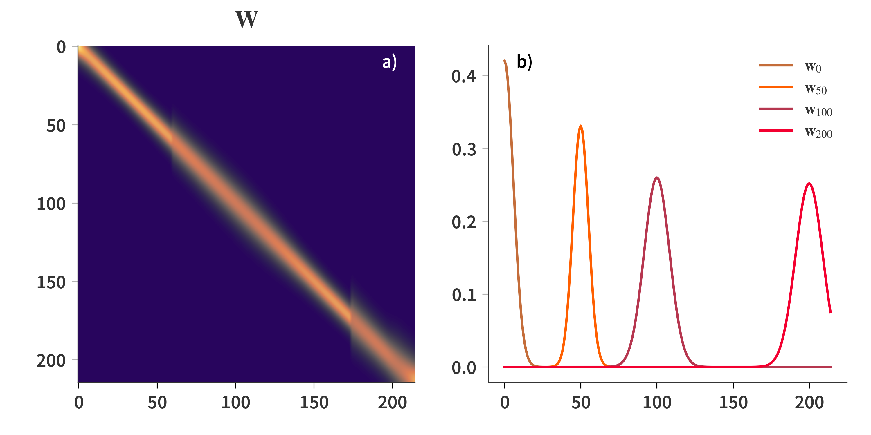
We’re now going to define the Gaussian dictionary, where each column consist of a single Gaussian with the FWHM predicted by Fig. 5b. Since a Gaussian is defined for each wavelength, and each having the same length as the spectral axis, the dictionary, $\mathbf{W}$, becomes square. The dictionary is depicted in Fig. 6. Notice here how the jumps in FWHM are clearly visible each time a new transmission order is introduced. Also remember that the columns of $\mathbf{W}$ are referred to as atoms. All atoms (the columns of $\mathbf{W}$) are normalized to $||\mathbf{w_i}||_2 = 1$.

Figure 6: a) Dictionary consisting of Gaussian atoms, with their FWHM being described by Fig. 5b. b) Some of extracted atoms from the dictionary.

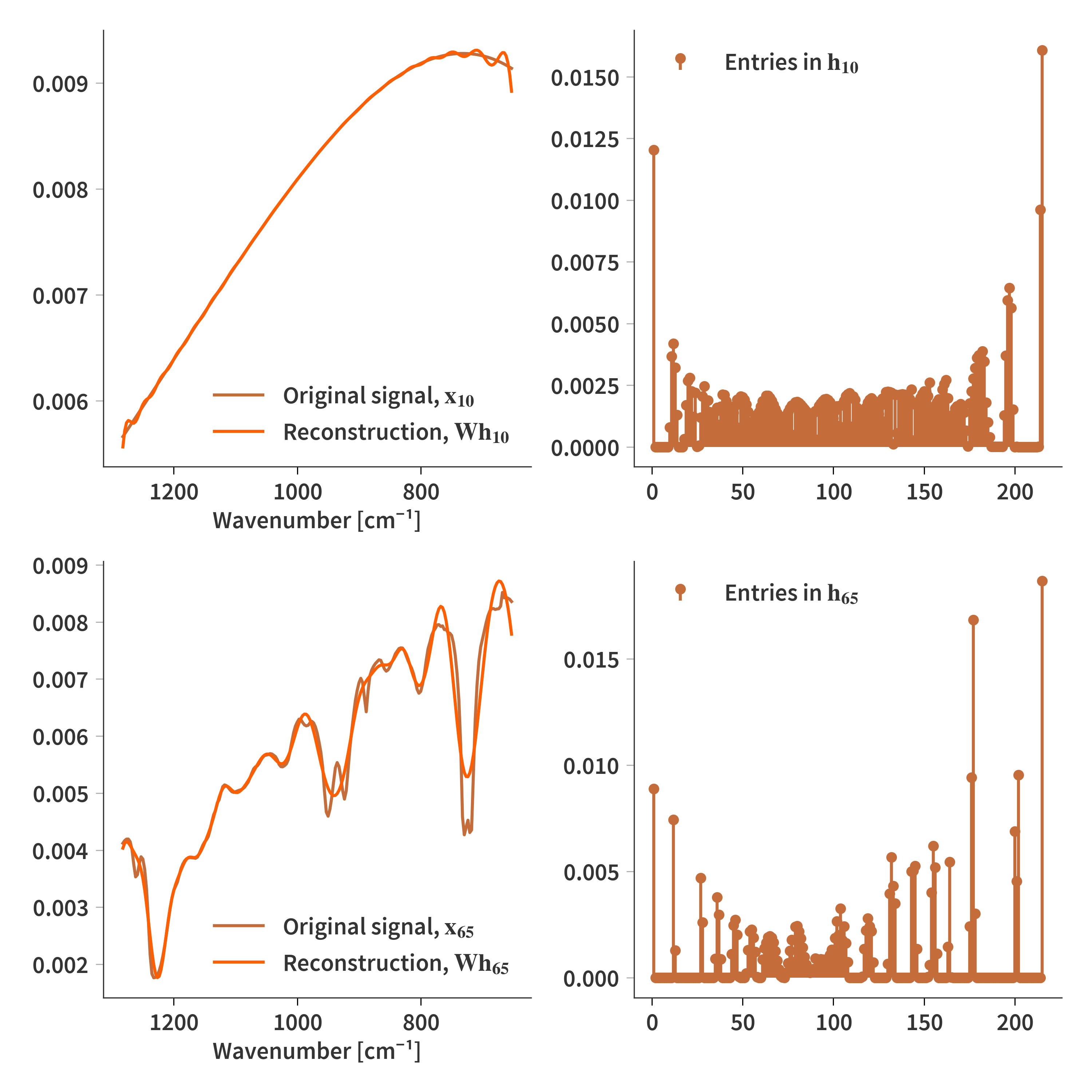
Now, we will look at the best case scenario: How well can a given signal be reconstructed using only this dictionary? We are going to use nonnegative matrix factorization for this and the minimization problem can therefore be expressed as:

\[\begin{align} \label{eq:arg_min} \arg \min_{\mathbf{H}} ||\mathbf{X} - \mathbf{WH}||_F^2 \quad \textrm{s.t.} \quad \mathbf{H} \geq 0 \end{align}\]

Where $\mathbf{X}$ is a matrix containing the signals we want to reconstruct in its columns. This can be solved using gradient decent, where the gradient of the cost function is

\[\begin{align} \label{eq:grad_H} \nabla_\mathbf{H}||\mathbf{X} - \mathbf{WH}||_F^2 = 2\mathbf{W}^T\mathbf{WH} - 2\mathbf{W}^T\mathbf{X} \end{align}\]

The update scheme of the gradient decent then becomes

\[\begin{align} \label{eq:update_H} \mathbf{H} \leftarrow \mathbf{H} - \alpha\left(\mathbf{W}^T\mathbf{WH} - \mathbf{W}^T\mathbf{X} \right), \qquad \alpha = \frac{2}{||\mathbf{W}^T\mathbf{W}||} \end{align}\]

This is implemented in the following python function, which utilize AN ACCELERATED DECENT STEP, WHICH I HAVE FOGOTTEN THE NAME OF AND WOULD LIKE A REFERENCE TO BY ANDERSEN ANG.

def fastGD_H(W, H, X, itermax):
    WtW = W.T @ W
    U, S, Vh = np.linalg.svd(WtW, full_matrices=True)
    stepsize = 1/S[0]
    WtX = W.T @ X
    
    cost_func = []
    
    V = np.copy(H)
    for i in range(itermax):
        grad_V = WtW @ V - WtX
        H_old = H
        H = np.maximum(0, V-stepsize*grad_V) 
        V = H + (i/(i+3)) * (H - H_old)
        cost_func.append(0.5*np.linalg.norm(W @ H-X)**2)
    return H, cost_func

Performing 1000 iterations of this algorithm yields the reconstructions which are presented in Fig. 7. Here, pretty good reconstructions are observed, while it is clear that the resolution of the Gaussians does inhibit the ability to reconstruct the finer details of the original signal. Also notice that larger deviations and oscillations can be observed at the edges of the signal.

Figure 7: Reconstructions of different signals based on a dictionary of Gaussians. THIS IS NOT RECONSTRUCTED INTERFEROGRAMS, BUT RATHER THE BEST OBTAINABLE RECONSTRUCTION OF THE INPUT SIGNALS BASED ON THE GAUSSIAN DICTIONERY. The coefficients of each reconstruction is indicated in the rightmost column.

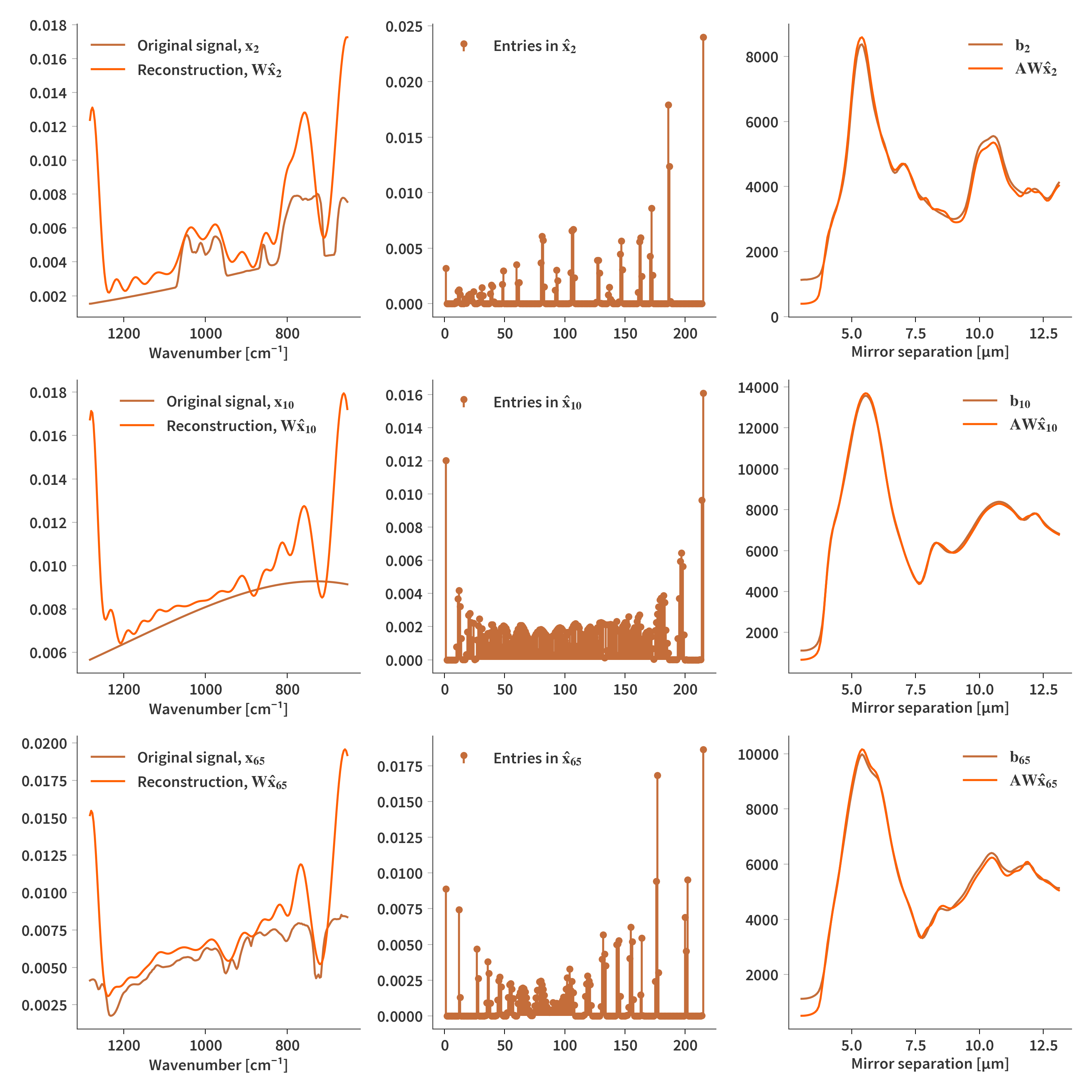
Now we have seen how good the reconstructions can potentially be, we are going to take a look at reconstructions of real signals from the interferometer. We’re going to solve (almost) the same problem as in Configuration 1 as stated in Eq. (\ref{eq:arg_min1}). Only here, we are going to ignore the offset, $\psi$ for a moment, and also, we can forego the smoothness regularization since the dictionary itself is already smooth. The reconstructed signal, $\mathbf{x}$, is however still subject to be nonnegative. That means that the new minimization problem can be written as

\(\begin{align} \label{eq:arg_min3} &\arg \min_{\mathbf{\hat{X}}} ||\mathbf{B} - \mathbf{AW\hat{X}}||_2^2 \quad \textrm{s.t.} \quad \mathbf{\hat{X}} \geq 0 \end{align}\) $\mathbf{B}$ contains all the interferograms in its columns, which allows us to perform all the reconstructions at once. If we introduce $\mathbf{\hat{A}} = \mathbf{AW}$ we can use the same solver as just used in the “best case” reconstruction and then simply get the true input spectra as $\mathbf{X} = \mathbf{W\hat{X}}$. Some examples are presented in Fig. 8, and the results are really not that pretty… And we need to figure out why It however looks like, the “reconstructed” interferograms look nice, so something else is going on… to be continued

Figure 8: Spectral reconstruction based on measured interferograms in the leftmost column. The middle column show the entries in $\mathbf{\hat{X}}$ and the rightmost column is the measured and calculated interferograms based on the solution of Eq. (\ref{eq:arg_min3}).