Chasing the system response matrix
Updated:
A reoccurring issue is not knowing the exact response matrix of the hyperspectral camera. This matrix should describe the relationship between the mirror separation of the scanning Fabry-Pérot interferometer (SFPI), the wavelength of the incident light and the output of the camera. Knowing this would aid in reconstructing the wavelength/wavenumber dependent spectra of the incident light, which at the moment are obscured and hidden in the interferograms.
I therefore set out to find this response matrix and will in the following document my attempts and findings.
We need data… this is how we get it
All of the experiments are going to be transmission measurements, since this gives the most well defined reference spectra. A black body radiator set to a given temperature gives a well defined emission spectrum given by the spectral exitance:
\[\begin{align} \label{eq:BB_exitance} M_{BB, \tilde{\nu}}(T) = 2\pi hc^2\tilde{\nu}^3 \frac{1}{\exp{\frac{hc\tilde{\nu}}{k_B T}} - 1}, \end{align}\]where $\tilde{\nu}$ represents the wavenumber given as the reciprocal of the wavelength $1/\lambda$, $h = 6.6261\times 10^{-34} \textrm{J}\cdot\textrm{Hz}^{-1}$ is the Planck constant, $c=2.9979\times 10^{8}$ m/s is the speed of light, and $k_{B} = 1.3806\times 10^{-23}\textrm{J}\cdot\textrm{K}^{-1}$ is the Boltzmann constant. Finally, $T$ denotes the absolute temperature of the black body. For more on black body radiation, click here.
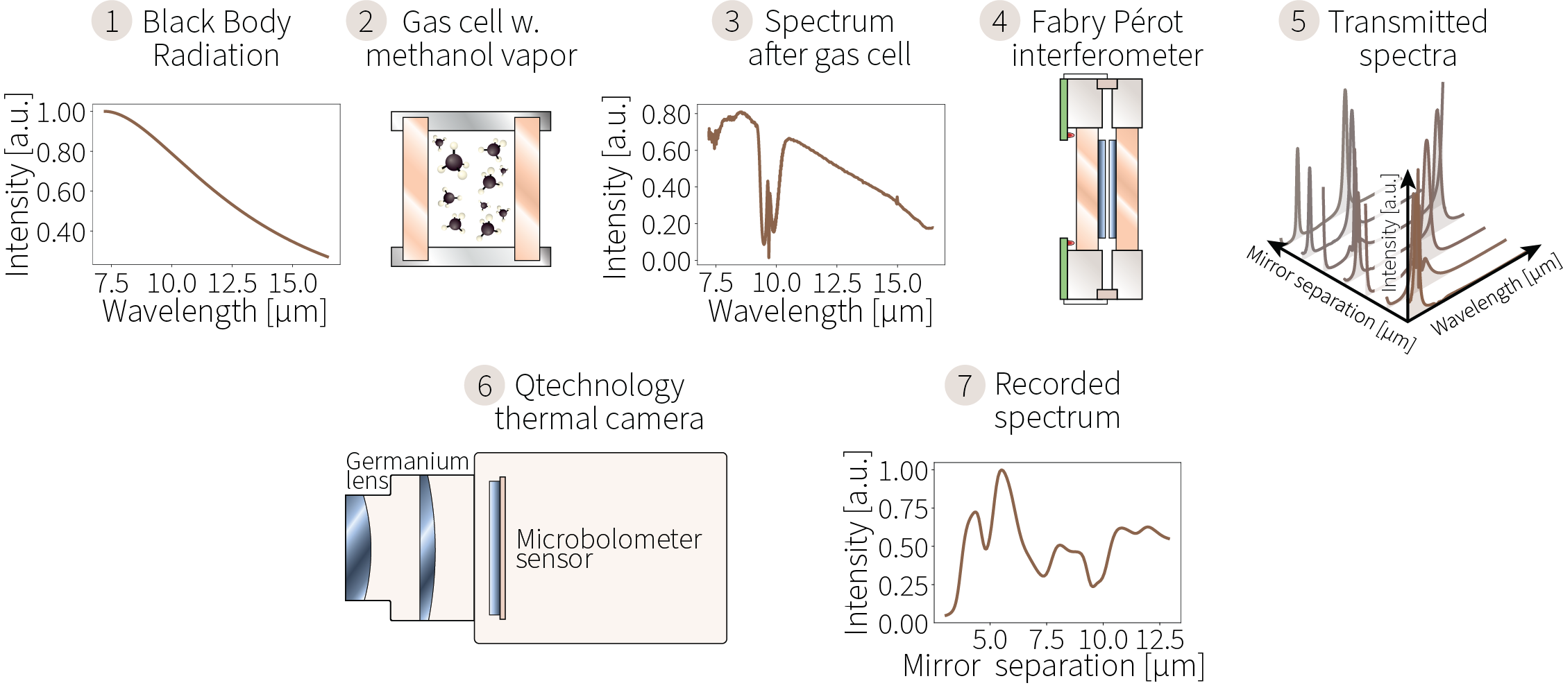
A black body radiation source is used in the lab and the precise spectrum can then be calculated from Eq. (\ref{eq:BB_exitance}). Because we’re working with transmission measurements, it is then possible to calculate the spectrum of the light incident on the SFPI as the product of the black body source and the FTIR transmission spectrum of the sample. Fig. 1 gives a schematic representation of how the black body spectrum firstly is transmitted through a sample (in this case a gas cell with methanol vapor, but i can be anything transmissive) and how it is converted to a interferogram as recorded by the hyperspectral thermal camera. In these experiments we are only going to consider light hitting the center of the microbolometer sensor to avoid dealing with spatial variations across the sensor and the spectral bending effects associated with light rays of non-perpendicular incidence.
46 of different materials have been measured as well the pure black body without any material in front of it. The camera is only sensitive in the range from ≈ 1250 cm-1, ($\lambda = 8$ µm) to ≈ 650 cm-1, ($\lambda = 15.38$ µm) but to make sure not to leave anything important out, data from 1300 cm-1, ($\lambda = 7.69$ µm) to 600 cm-1, ($\lambda = 16.67$ µm) is included. The FTIR spectra of all materials can be found here. The light incident on the SFPI is found as the product of the black body emission given by Eq. (\ref{eq:BB_exitance}) and the FTIR transmission spectrum as depicted by Fig. 2. Some of the materials are imaged multiple times at different black body temperatures, and the interferograms of every single measurement (114 in total) are depicted here along with the exitance spectra here.

Data preprocessing
An inherent challenge of the hyperspectral camera is the fact that at no point during the image capture, do we know the absolute mirror separation. We only know the relative displacement of the mirrors based on the interferograms of three laser diodes mounted around the mirror perimeter. To solve this we need to have a spectral reference point which all data cubes can be aligned to. For this, a 8.226 µm bandpass filter is placed in front of a hot plate set to ≈ 75 ºC. Both are positioned in the frame to be just above the black body. The SFPI goes through three transmission orders during the sweep, and the second (middle) order is used for the alignment. This is “defined” to occur at a mirror separation (MS) of 8.13 µm. The spectral resolution of the data cube is note necessary high enough to capture the exact position of the maximum of the 2nd transmission order. The central peak is therefore fitted with a Gaussian with 10 times more data points compared to the number of spectral channels in the data cube. The relative displacement which is calculated based on the laser diode interferograms is then offset until the position of the fitted Gaussian aligns with an MS of 8.13 µm. The wavelength of the laser diodes have been experimentally determined to be 680 nm.
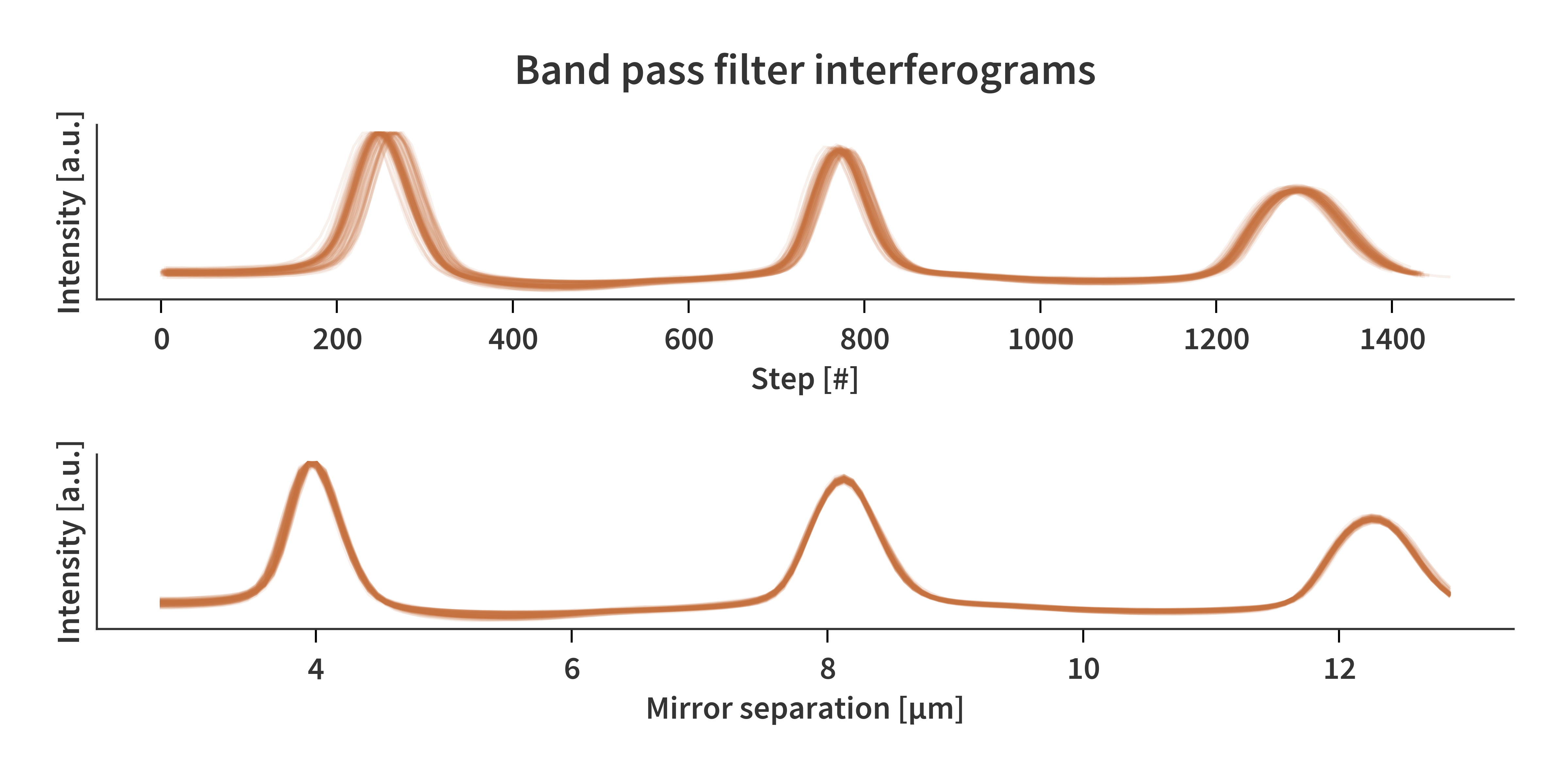
Fig. 3 illustrates the interferograms before and after the alignment. Apart from the alignment of spectral axes, the camera also does not save the same number of spectral channels in each cube. This means that when all data cubes have been loaded and spectrally aligned, they must be interpolated along the MS axis. A linear scale is chosen with its starting value corresponding to the highest “initial MS” in the data set, and similarly the end point is chosen to correspond to the lowest “final MS”. The number of interpolation points is chosen to correspond to the lowest number of spectral channels across the data set, which usually is ≈ 150. Only now are we able to compare measurements across data cubes and we can continue with our journey towards the perfect fit.
############################################################################
MORE DETAILS AND ILLUSTRATIONS ARE NEED FOR THIS PART AS WELL AS MORE OBJECTIVE EVALUATION OF THE PERFORMENCE OF THIS METHOD
############################################################################
Solving for the system matrix
My initial attempt to find the response matrix is by turning it into a least squares problem. The unknown system matrix is described by the matrix $\mathbf{A}$, the spectra of the incident light is stored as the columns of the matrix $\mathbf{X}$, and the recorded interferograms are represented by the columns of the matrix $\mathbf{B}$. The problem can therefore be formulated as
\[\begin{align} \label{eq:AXB} \mathbf{AX} = \mathbf{B}, \end{align}\]where we want to solve for $\mathbf{A}$.
The known matrices are represented graphically in Fig. 4
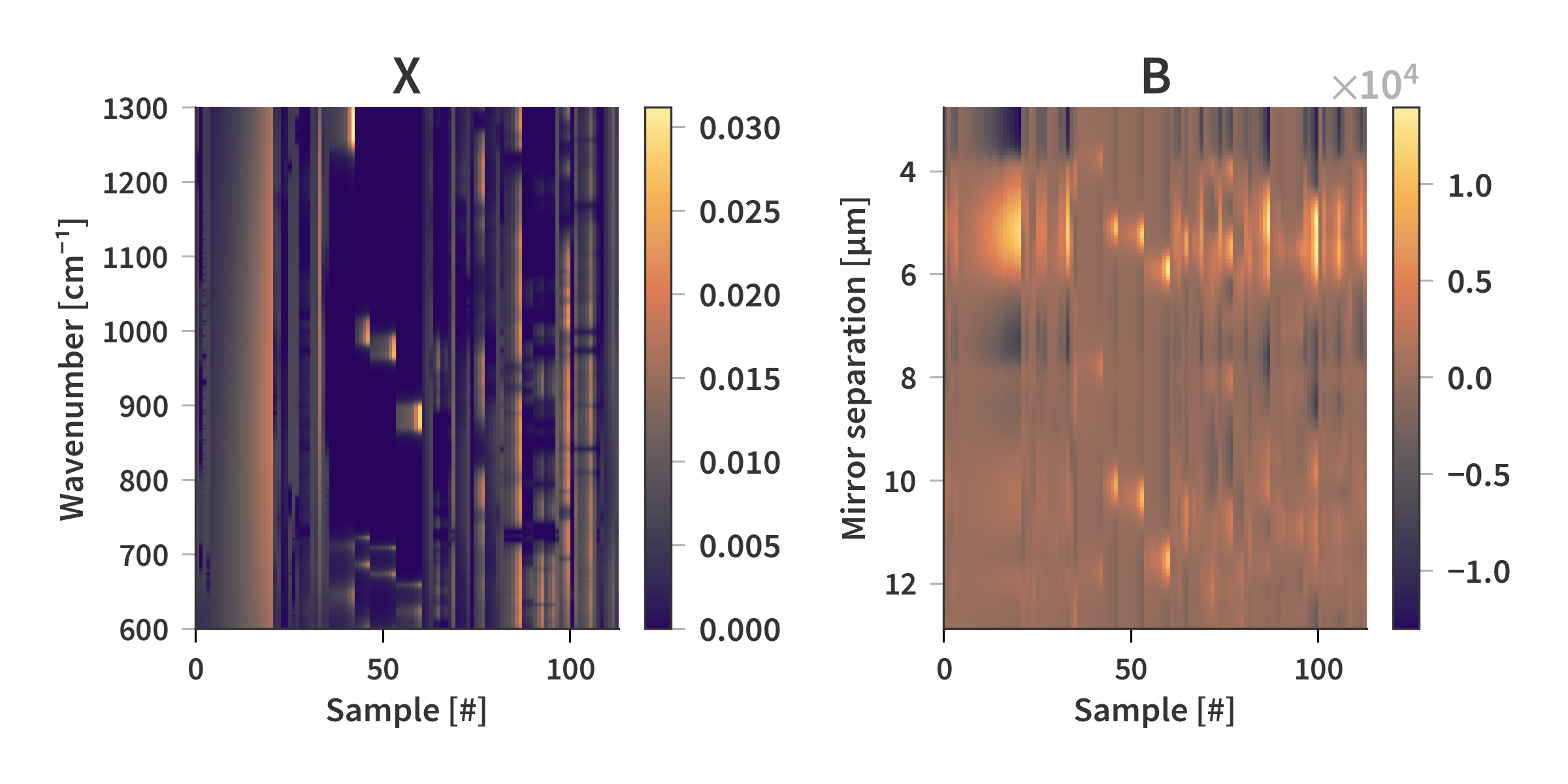
This system is hugely under-determined as the number of rows in $\mathbf{X}$ is 2801, and the number of rows in $\mathbf{B}$ is ≈ 150 (The camera simply captures as many images as it can during a sweep, and the total number changes from run to run). The dimensions of $\mathbf{A}$ then becomes $m\times n = 2801\times 150$ which means that there are many more variables to solve for compared to the number of equations. Finding a solution is not a problem since there are an infinite number of solutions satisfying $\mathbf{AX} = \mathbf{B}$, but finding a solution which is physical and can be used for other spectra not in the data set turns out to be quite a challenge. To give the solver the best chance of finding a satisfactory solution we are going to need as many different samples as possible covering as large a part of the spectrum as possible.
However, we are working completely blind when it comes to finding a realistic solution of $\mathbf{A}$. The Airy function can be used to calculate the transmission of a theoretical SFPI for any given combination of mirror separation and wavelength.
\[\begin{align} \label{eq:airy} \Gamma = \frac{1}{1 + F\sin^2{2\pi d \tilde{\nu}}} \end{align}\]Here, $\Gamma$ is the transmission of the SFPI at the mirror separation $d$ and wavenumber $\tilde{\nu}$. $F$ is the coefficient of finesse defined as
\[\begin{align} \label{eq:F} F = \frac{4r^2}{(1-r^2)^2}, \end{align}\]with $r$ being the reflectance of the mirror. In this case the mirrors have a reflectance of $r = 0.8$ resulting in $F=19.75$. The airy function reaches a maximum of 1 whenever $2\pi d \tilde{\nu} = m \pi$ where $m = 0, 1, 2, \dots$. The conditions for transmission can therefore be expressed as
\[\begin{align} \label{eq:transmission_condition} d = \frac{m}{2\tilde{\nu}}, \qquad d = m \frac{\lambda}{2}, \qquad \lambda = \frac{2}{m} d, \qquad \tilde{\nu} = \frac{m}{2d} \end{align}\]Fig. 5 shows the transmission calculated using the airy function in Eq. (\ref{eq:airy}) for all combinations wavelengths and mirror separations in this study.
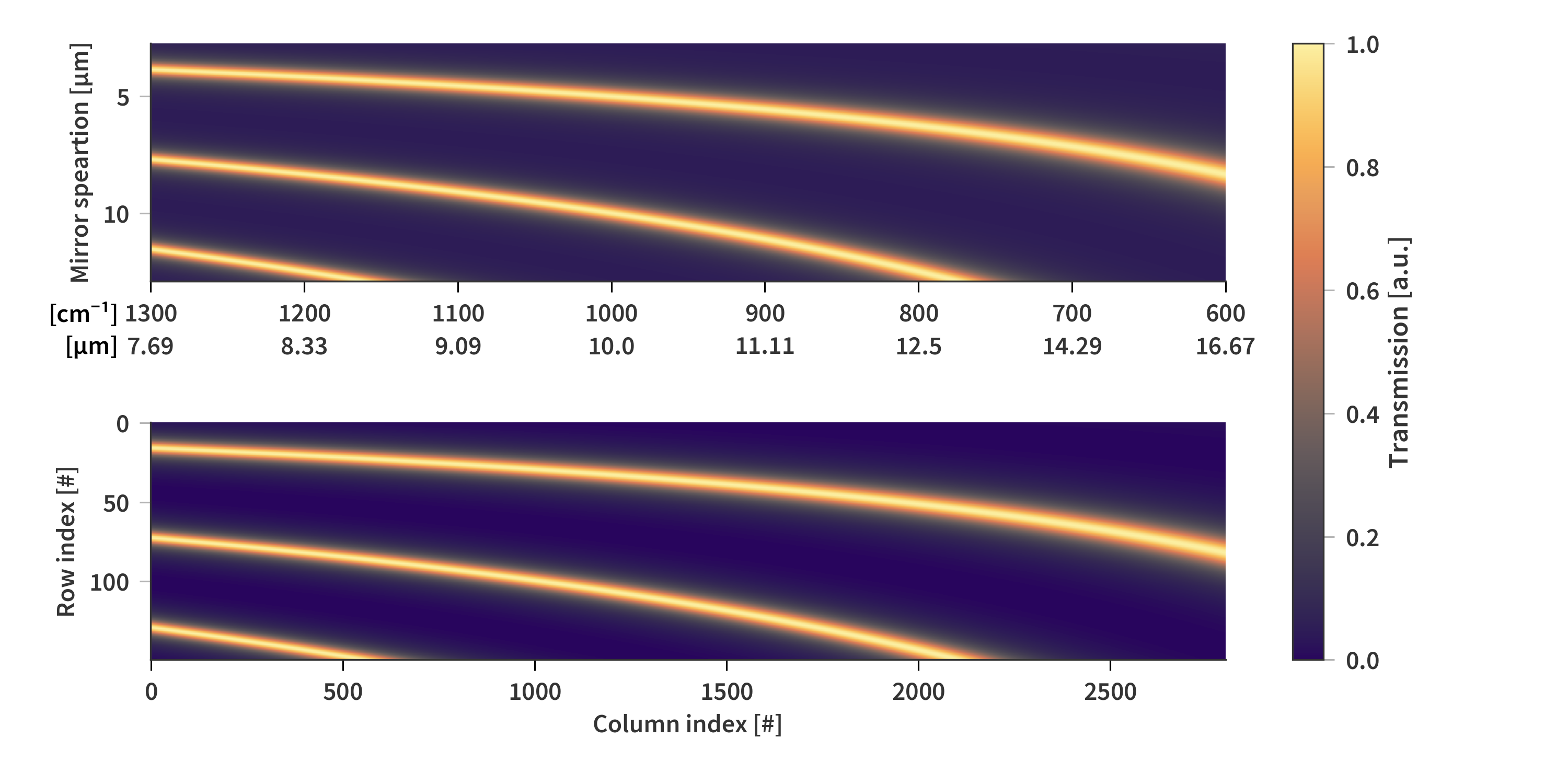
The airy function can serve as a good initial estimate for $\mathbf{A}$. The objective function we are trying to minimize can therefore be written as follows
\begin{align} \label{eq:cost_function} \textrm{minimize:}||\mathbf{AX} - \mathbf{B}||^2 + \gamma ||\mathbf{A} - \mathbf{\hat{A}}||^2, \end{align}
where $\mathbf{\hat{A}}$ is the initial guess for a solution, and $\gamma > 0$ is a regularization parameter.
As described in this Stack Exchange post, it is possible to solve the problem directly using
\[\begin{align} \label{eq:direct_solve} \mathbf{A} = (\mathbf{B}\mathbf{X}^T + \gamma_{init}\mathbf{\hat{A}})(\mathbf{X}\mathbf{X}^T + \gamma_{reg} \mathbf{M})^{-1} \end{align}\]where $\gamma_{init}$ and $\gamma_{reg}$ are regularization parameters for weighting the initial guess and regularization matrix $\mathbf{M}$ respectively. In the most basic case, $\mathbf{M}$ is usually set to the identity matrix, $\mathbf{I}$. However, this yields some pretty bad - or at least nonphysical - results. Fig. 6 shows solutions to $\mathbf{A}$ based on Eq. (\ref{eq:direct_solve}) with different values of $\gamma_{init}$ and $\gamma_{reg}$.
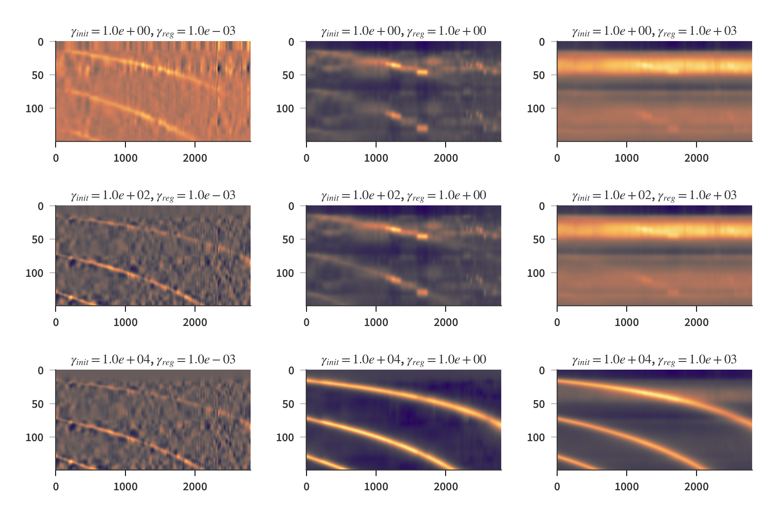
To no surprise it appears that a larger $\gamma_{init}$ leads to the final solution resembling the Airy function more closely. There are however some slight differences in their shape. Notice how the 2nd order of the Airy function “terminates” just above column 2000. This is also the case for all of the calculated solutions of $\mathbf{A}$ except the one with $\gamma_{init} = 1 \times 10^0$ and $\gamma_{reg} = 1 \times 10^{-3}$. Here the second order crosses the border slightly below column 2000. Also, the orders do no reach the edges as for the rest of the solutions. This is to be expected of the true solution, as the camera is not sensitive to all the wavelengths included in the data.
Random starting guess
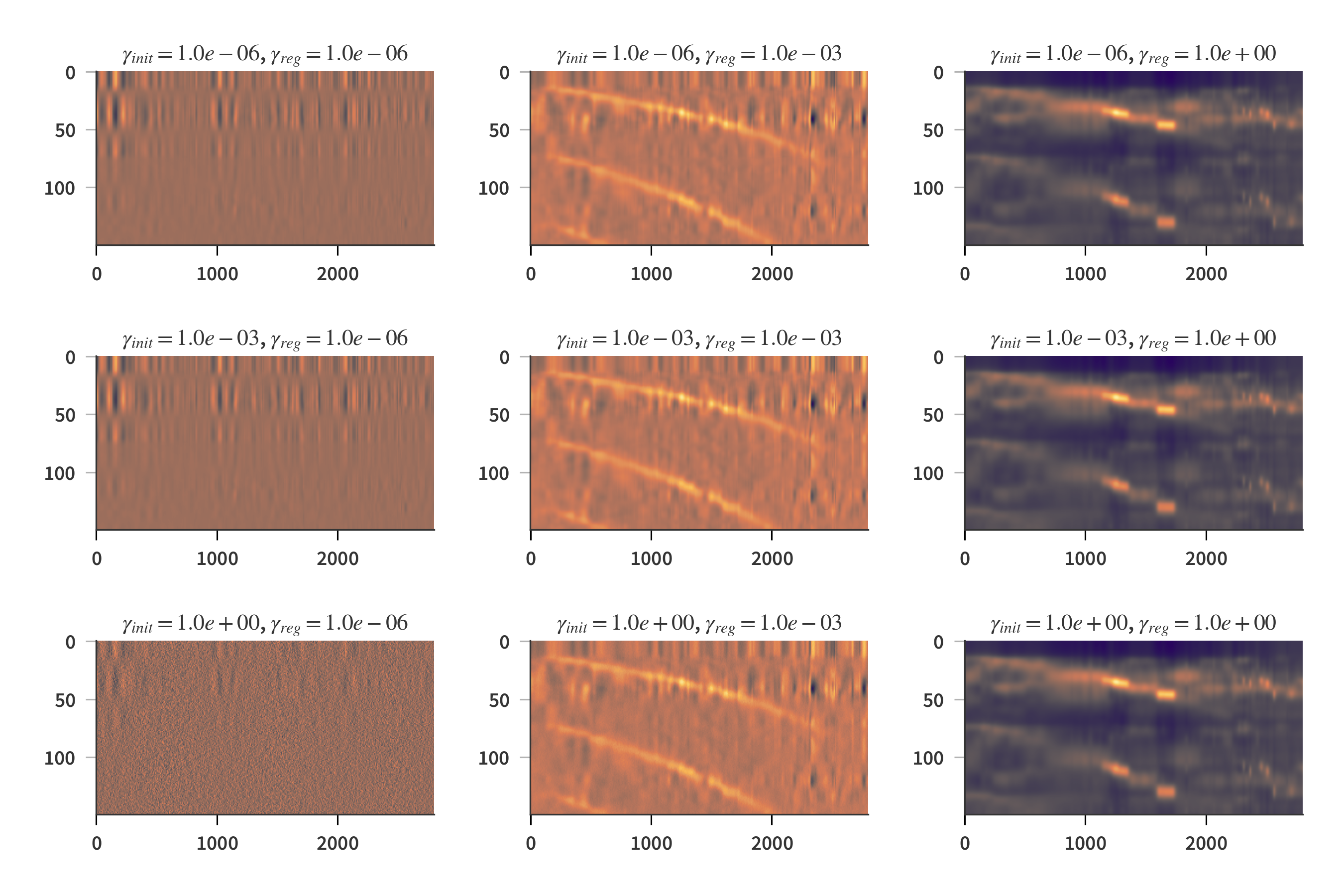
I would therefore like to see, if it is possible to find a solution which resembles the Airy function even without including it as the initial guess. Fig. 7 shows solutions of $\mathbf{A}$ for different values of $\gamma_{init}$ and $\gamma_{reg}$, but this time with a random initial guess. Now it is actually possible to find a solution to the problem which is reminiscent of the Airy function - even without providing it to the solver in the first place. It is however also evident that the solutions are quite sensitive to the choice of regularization parameters.
Random starting guess and new regularization matrix
Another regularization matrix is introduced and has the form of
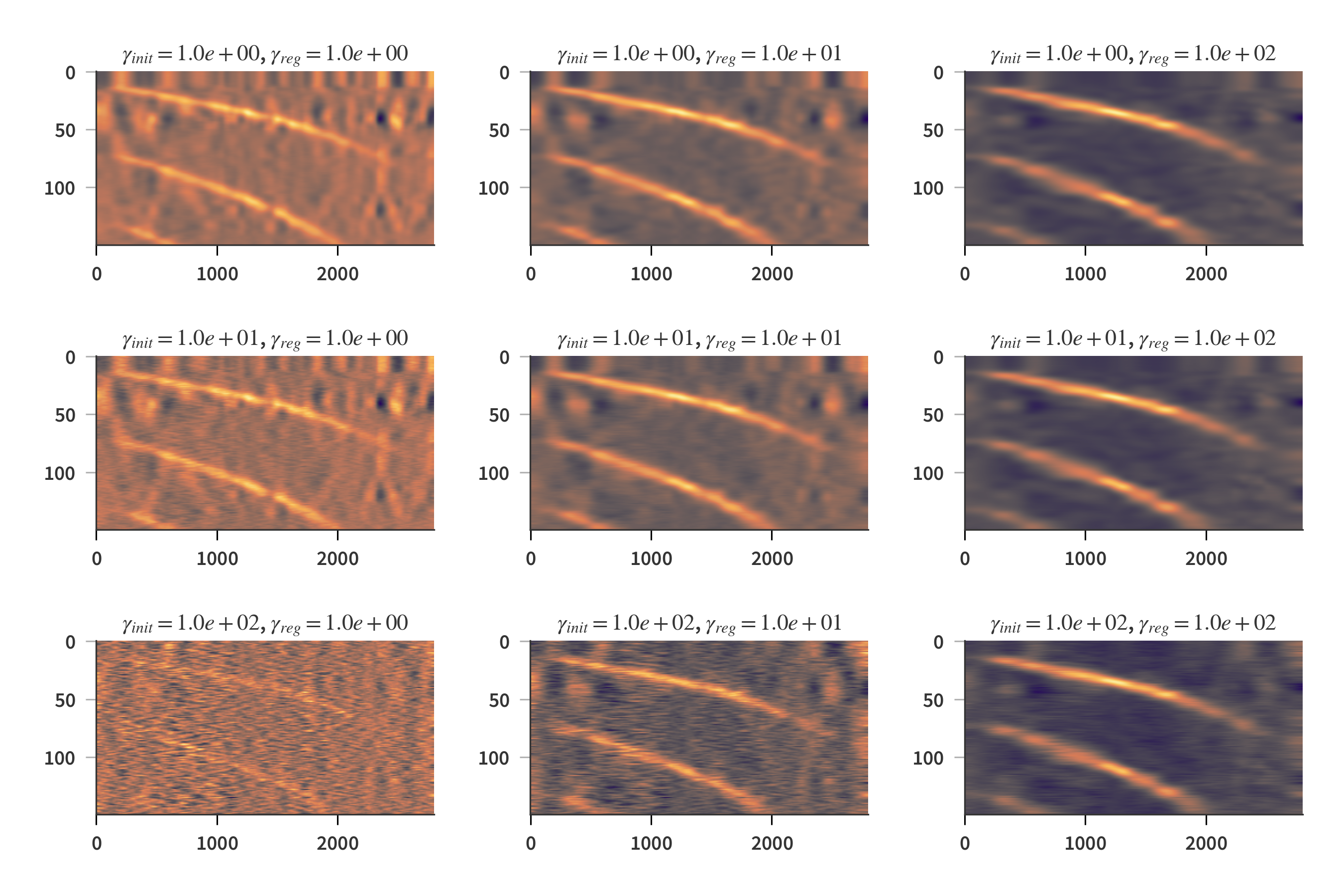
\[\begin{align} \label{eq:M_reg} \mathbf{M} = \begin{bmatrix} 1 & -1 & 0 & 0 & 0 & \dots \\ -1 & 2 & -1 & 0 & 0 & \dots\\ 0 & -1 & 2 & -1 & 0 & \dots\\ \vdots & \ddots & \ddots & \ddots & \ddots & \ddots\\ \dots & 0 & 0 & -1 & 2 & -1\\ \dots & 0 & 0 & 0 & -1 & 1\\ \end{bmatrix} \end{align}\]This form of regularization aims to suppress oscillations in the solution along the “x-axis” as it is derived from the 2nd order difference method. Roughly speaking it states that if we are looking at the $j^\textrm{th}$ element in the $i^\textrm{th}$ row of $\mathbf{A}$, then $-\mathbf{A}_{i, j-1} + 2\mathbf{A}_{i, j} - \mathbf{A}_{i, j+1} = 0$. Then the higher the value of $\gamma_{reg}$, the stronger this constraint is enforced. Fig. 8 show the results using this type of regularization and appears to giv a result closer to what is expected compared to when using the identity matrix for regularization.
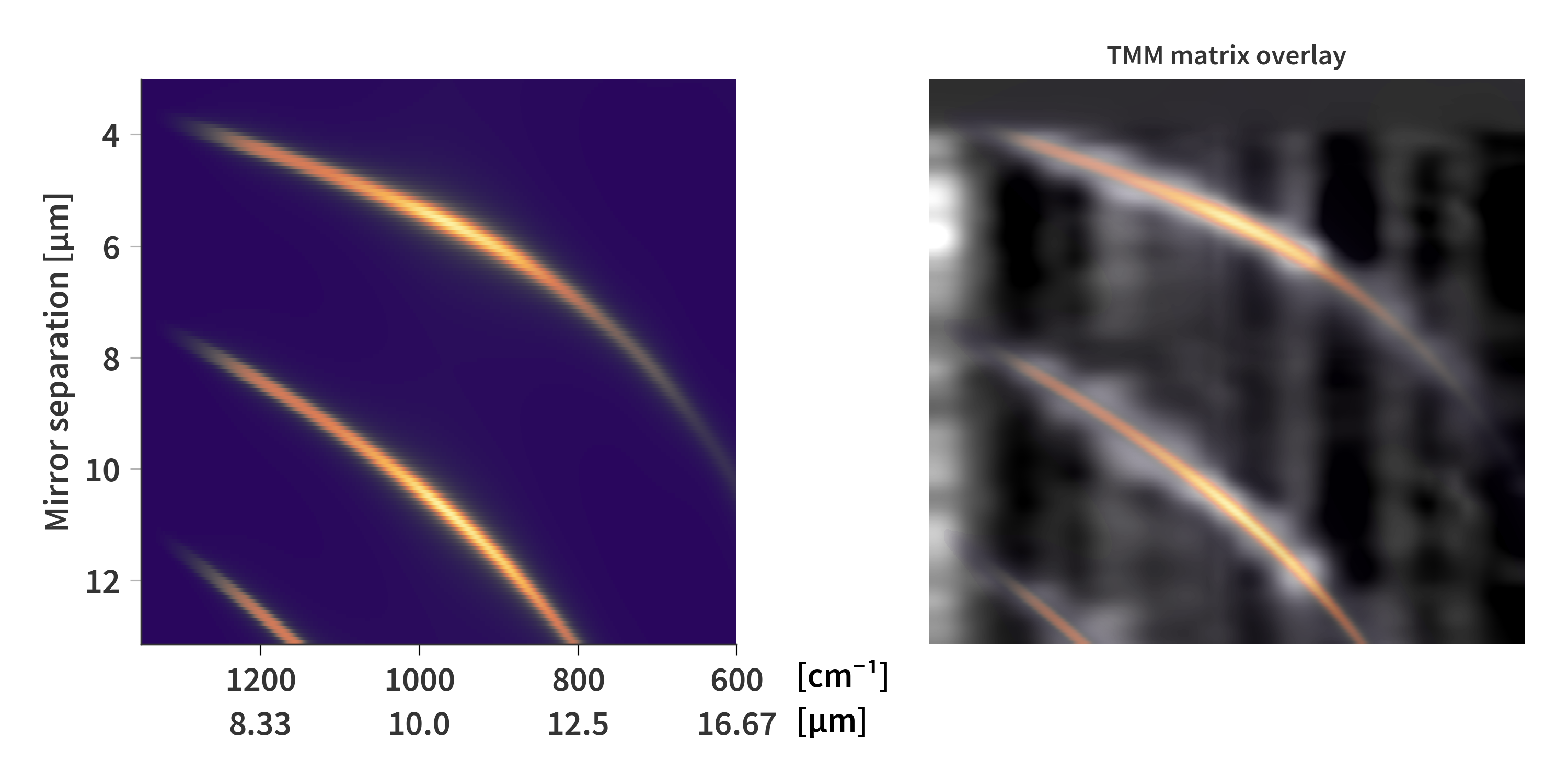
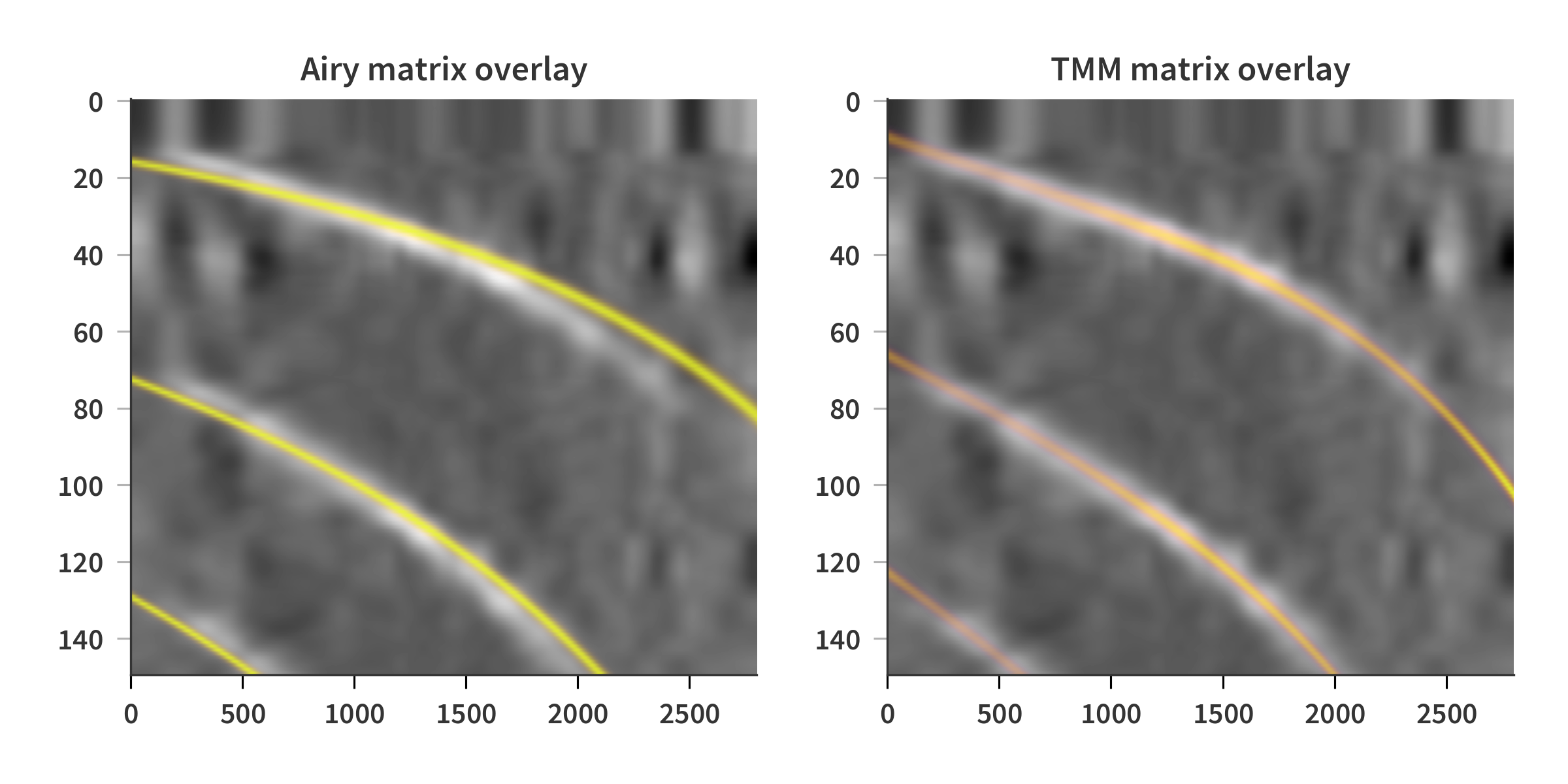
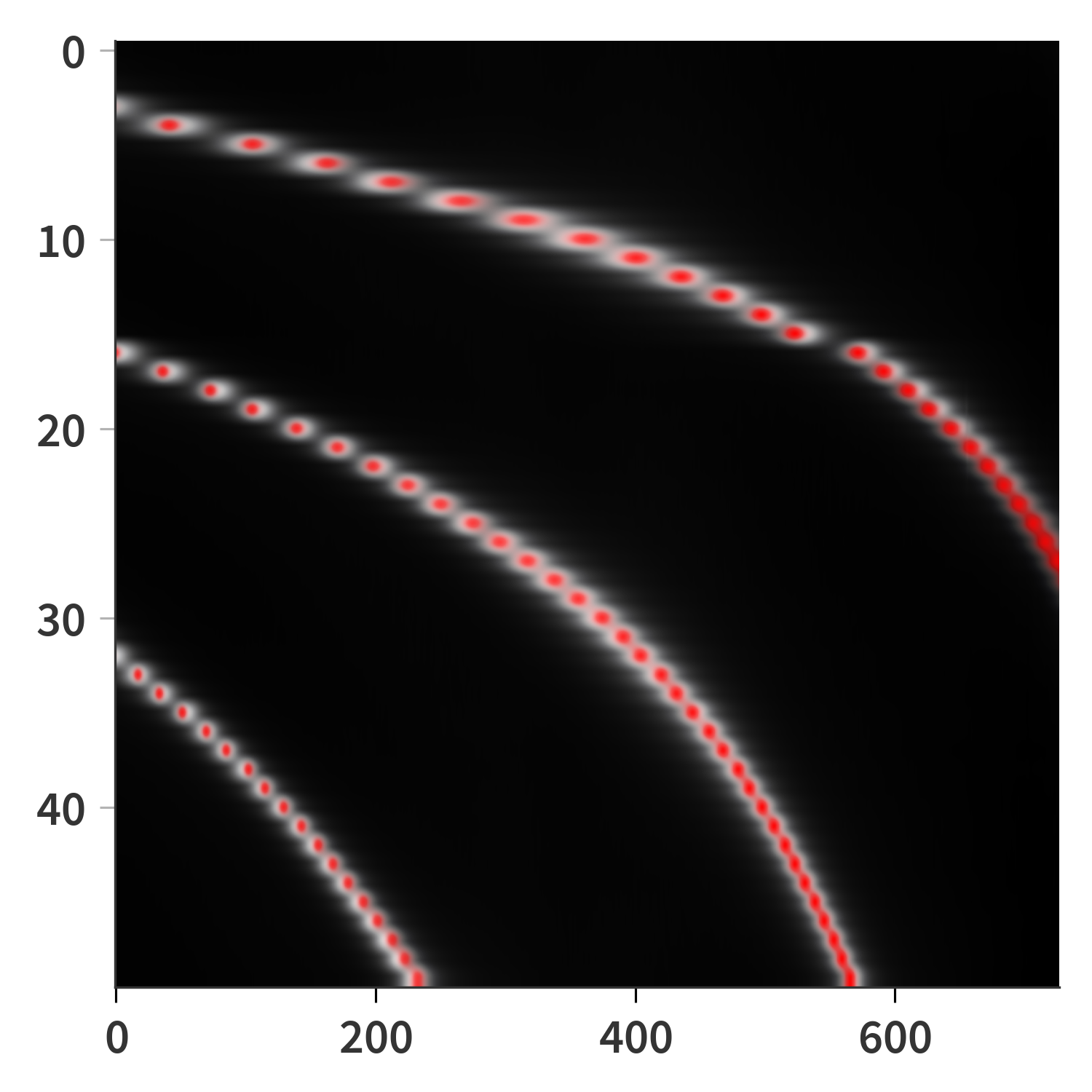
So it is possible to find a solution which comes close to what is expected theoretically. But how close is it actually. Some deviation from theory are to be expected, but to get a better feeling for how different the solutions are, I have overlaid the Airy matrix on top of one of the solutions for $\mathbf{A}$ with a random initial guess (Fig. 9). I have also found a theoretical solution using the transfer matrix method (TMM) as described in more detail here. The least squares solution has been plotted in gray-scale, while only the maxima of the theoretical matrices are displayed in color. Notice here, that there is almost a perfect fit between the TMM matrix and the solution, whereas the Airy matrix in comparison deviates much more. This indicates that the TMM estimate is actually quite close to what would be the true solution.
Can’t we just measure it using FTIR?
Wouldn’t it be nice if we could just measure the response of the SFPI directly and then worry about the sensor response later? An obvious solution is to throw the SFPI into an FTIR and then measure its transmittance at several different mirror separations. But (and there always is a ‘but’) one of the main problems with this that we do not know the absolute mirror separation distance. Secondly, controlling the piezo actuators in small steps and then maintaining their position also turns out to be quite a challenge (Fig. 9). I pieced together a python GUI which makes it possible to control the mirrors and can be downloaded here.
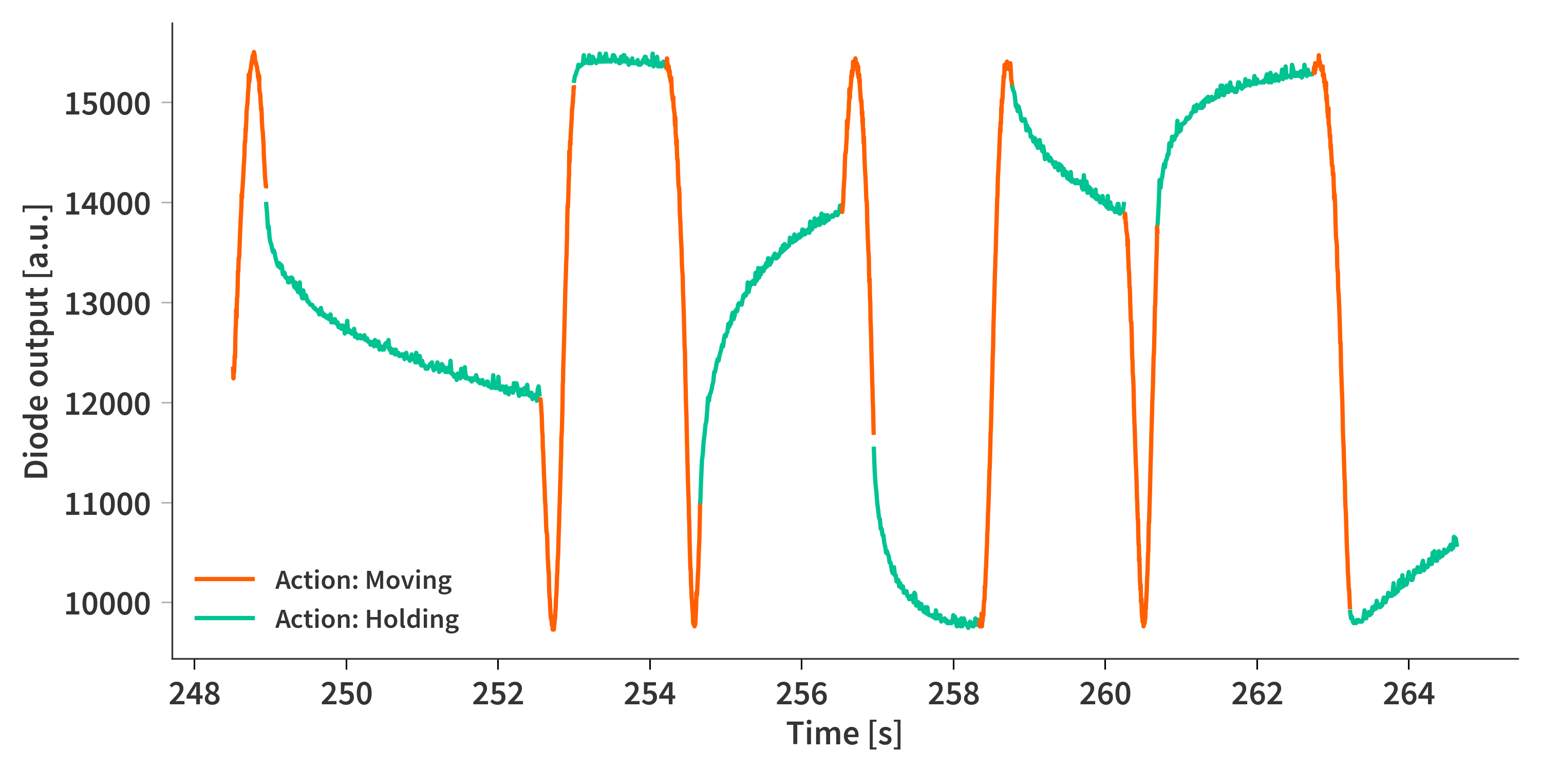
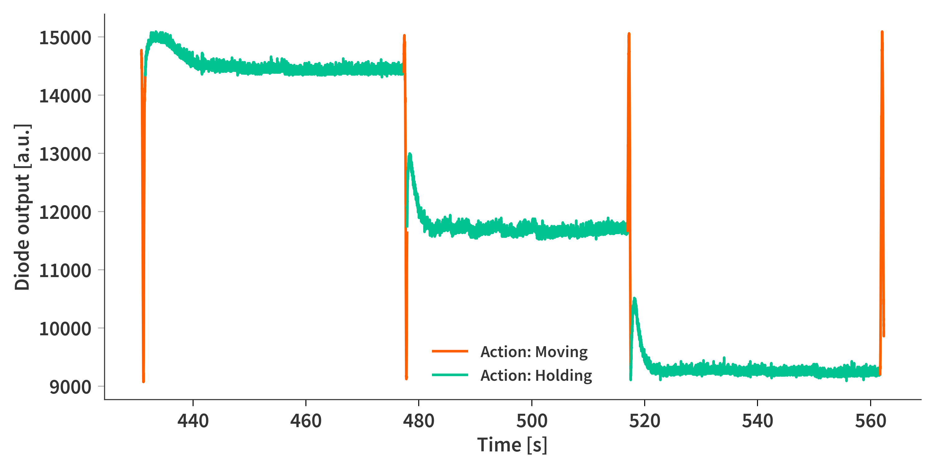
The piezo expansion is controlled by applying a voltage to all three actuators. When employed in the camera, this voltage is unique to each piezo to ensure they all expand the same amount. This is not that much of an issue here even though it would be nice, but the effect is assumed to be of minor importance here. Instead the same voltage is simply applied to all three at once. The next thing is maintaining a certain separation while performing the FTIR measurement. A PID-controller is implemented in the code where the outputs of the photo diodes are monitored while the mirrors are supposed to be held steady (Fig. 10). This makes it possible to perform minute adjustments to ensure that they do not drift from their previous position. This is however not perfect and the controller sometimes gets ‘confused’ and instead moves the mirror by an additional fringe (usually that means further apart).
How far have the mirrors moved between measurements
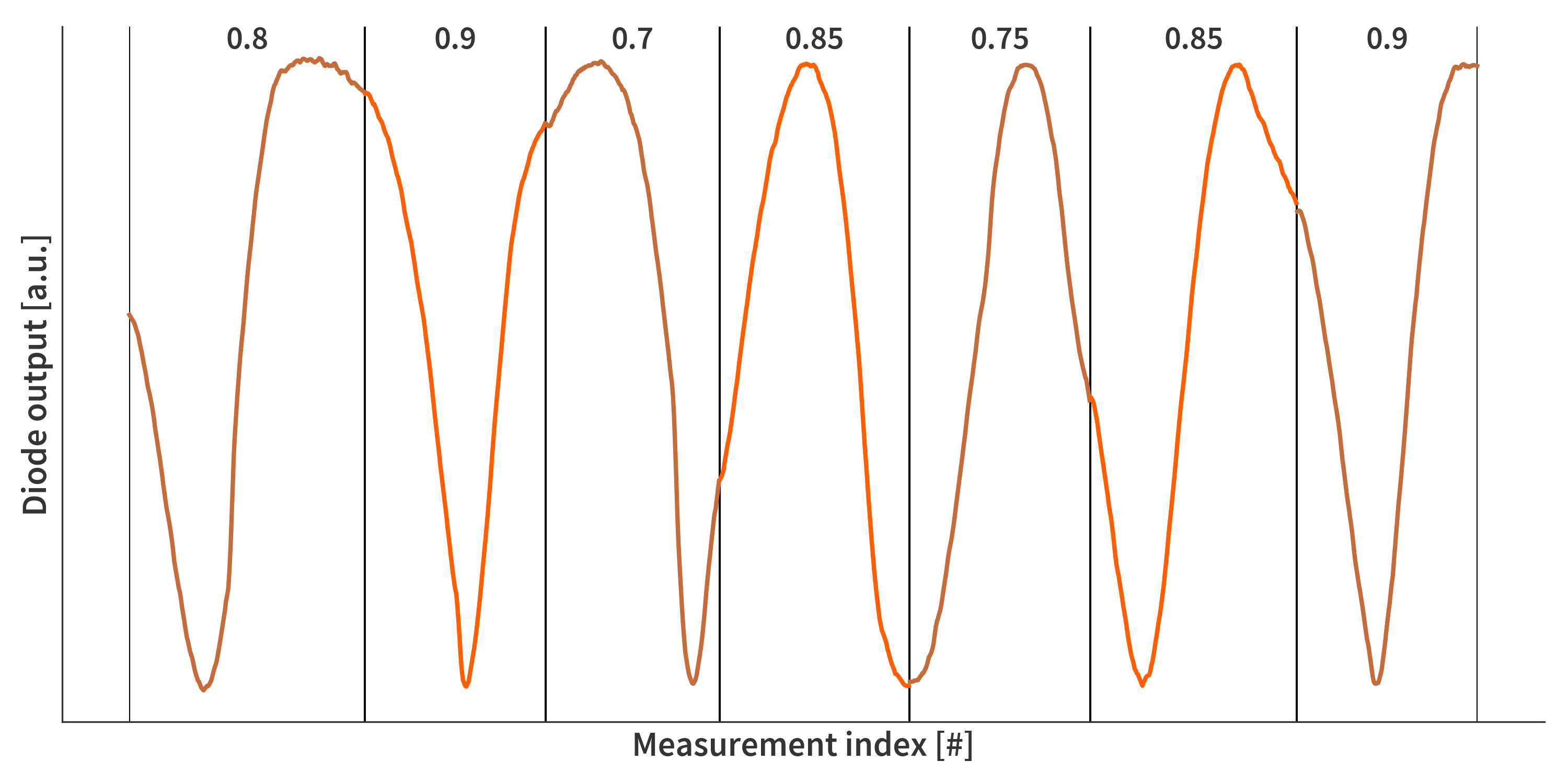
One would think that I would be rather straight forward to look at the diode interferograms and give a precise estimate of how far the mirrors have moved… At least that is what I thought. However, almost always, the mirrors are displaced less than a complete period which make automatic fitting procedures quite unreliable. Also, the interferogram is not quite a sine curve… rather it is based on the Airy function (Eq. \ref{eq:airy}). I spend a long time trying to automate this, but ended up painstakingly sitting and giving my best guess for every single step (Fig. 11). Luckily, every so often, the end of a step lines of with either a peak or a trough which means I am able to ‘check’ my estimates along the way. I do this for each of the three diodes such that I end up with a list of how far each piezo displaces the mirror at each step. The average of all three diodes is then used as the measure for the entire SFPI as a whole. It is assumed that the effective wavelength (combination of wavelength and angle of reflection) is the same for all three laser diodes ($\lambda_\mathrm{eff} = 686$ nm). Moving the mirrors $\lambda_\mathrm{eff}/2$ further apart will cause the diode interferogram to move a single period. Knowing this it is possible to calculate the relative displacement of the mirrors based on the fractional fringed counted at each step.
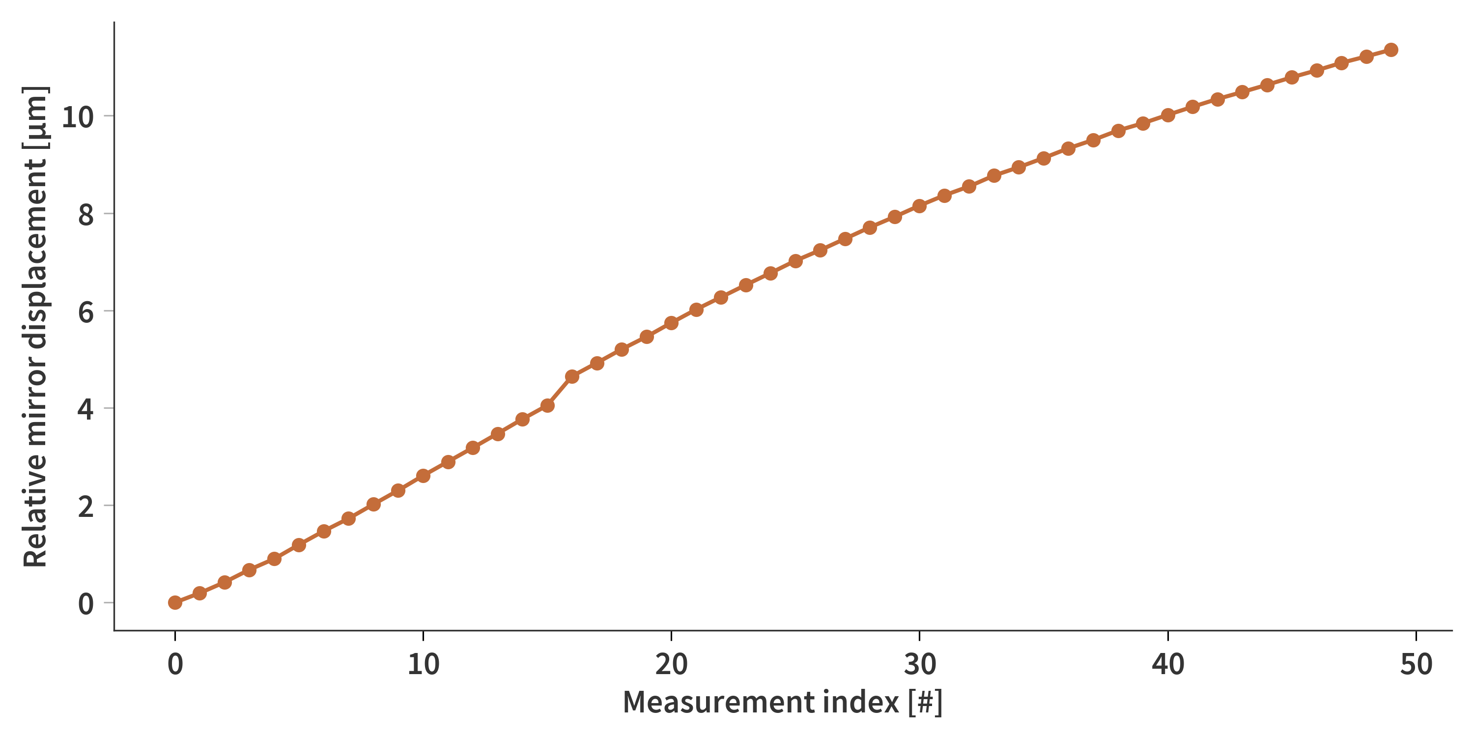
Based on the output from the photo diodes it is possible to construct the curve in Fig. 12, which illustrate how much the mirrors are displaced during each step. The sudden jump at index 17 is due to a missing measurement.
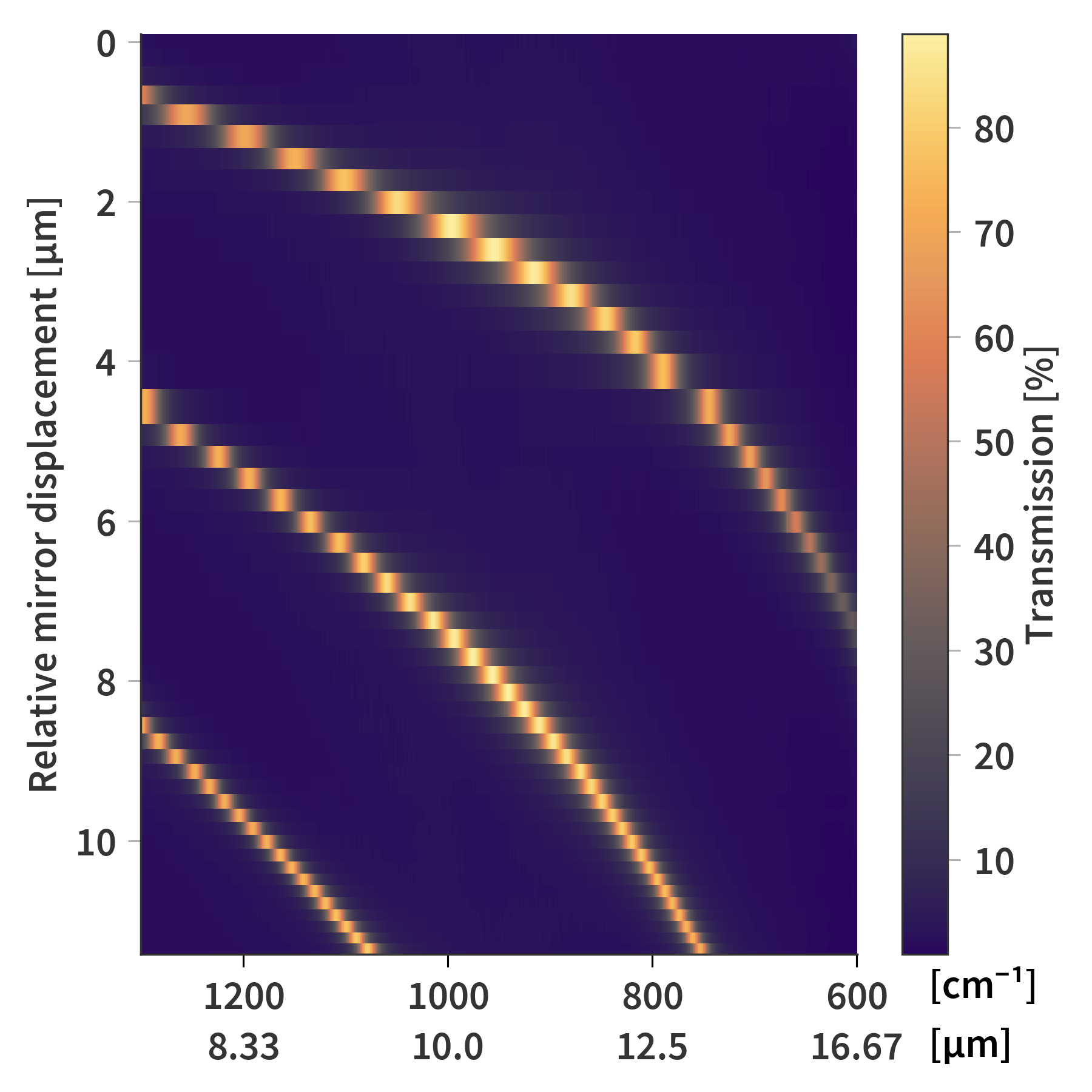
We also have the FTIR measurement at each mirror position (Fig. 13). Each row represents a single FTIR transmission spectrum (only in the range from 600 to 1300 cm-1) taken at a given mirror separation. Each row is associated with a certain relative mirror separation based on Fig. 12.
But HEY! Isn’t it possible to calculate the absolute mirror separation from the FTIR spectra directly? I’m glad you asked because it is… sort of (There’s that ‘but’ once again).
Let’s start out by looking at the conditions for maximum transmission based on Eq. (\ref{eq:transmission_condition}). From here we can get:
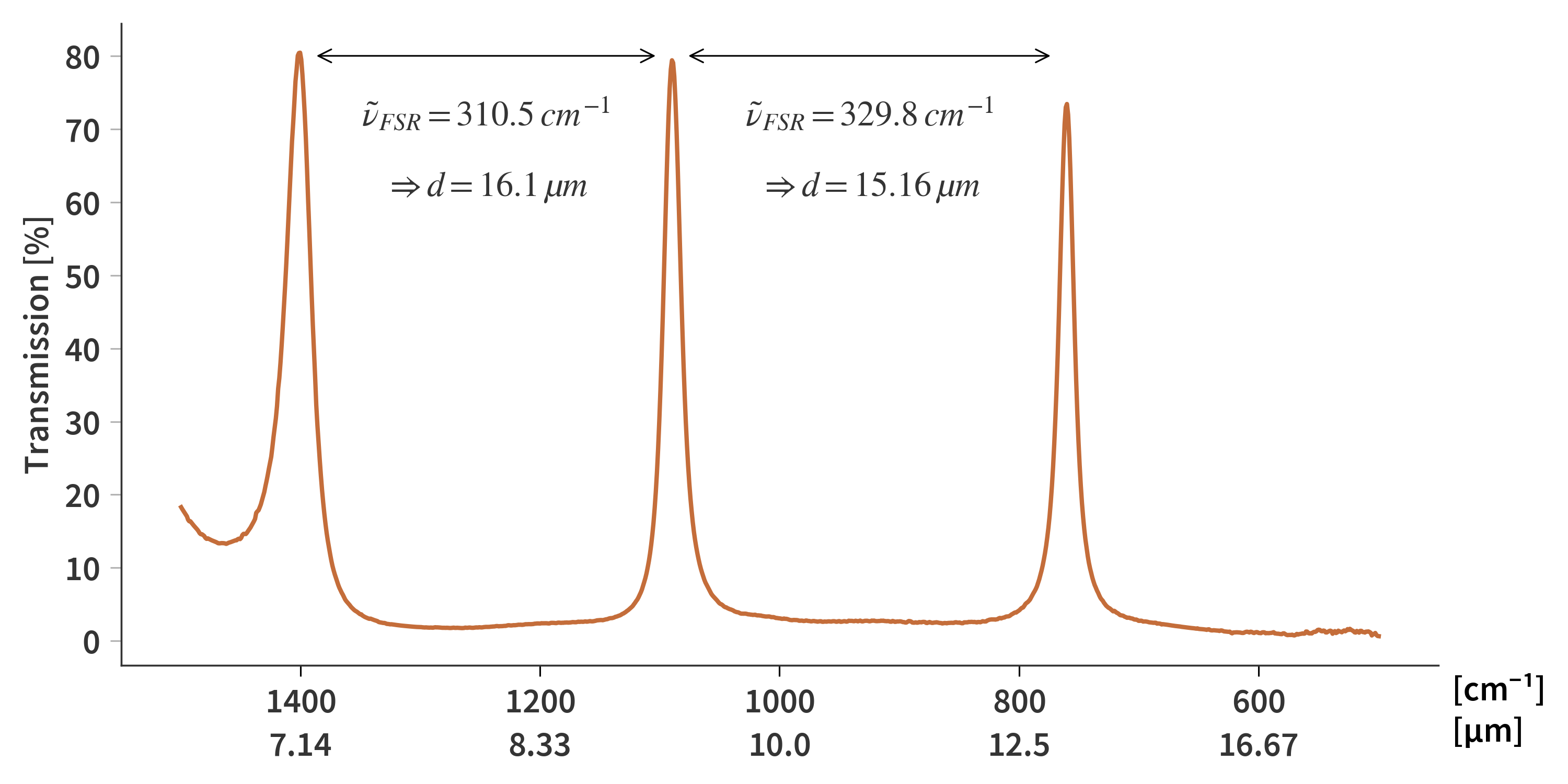
\[\begin{align} \label{eq:k_fsr} &m = 2d\tilde{\nu} \\[1.1em] \Rightarrow & \frac{m + 1}{\tilde{\nu} + \tilde{\nu}_\textrm{FSR}} = 2d \\[1.1em] \Rightarrow & d = \frac{1}{2 \tilde{\nu}_\textrm{FSR}}, \end{align}\]where $\tilde{\nu}_\textrm{FSR}$ is the “Free Spectral Range” of the SFPI - the distance (measured in cm-1) between two neighboring peaks. This means that the peaks are equidistant (again measured in cm-1) at a given mirror separation, $d$. If we then measure the distance between peaks, we should be able to derive the absolute mirror separation. But here is the issue: We are working with dielectric mirrors - that is, their reflectance vary across the spectrum. This effect is seen in Fig. 14 where the $\tilde{\nu}_\textrm{FSR}$ is measured twice across the spectrum. In this case I have allowed myself to increase the range to include parts of the spectrum which have previously not been included as the camera sensor is not sensitive in these regions. Nonetheless, this illustrates the effect that the $\tilde{\nu}_\textrm{FSR}$ decreases with shorter wavelengths. This results in the mirror separation distance being estimated longer than it actually is. This effect is also predicted by the TMM calculations so it is not simply due to a broken calculator (nor broken fingers). As mentioned previously, this is caused by the mirrors being dielectric rather than metallic. The ‘plane of reflection’ changes with wavelength due to changing refractive indices. This is therefore not a reliable way of predicting the absolute mirror separation.
Comparing the FTIR measurements to TMM calculations reveal good agreement between measurements an theory. However once again it is difficult to match the exact peak positions across the entire wavelength range. Also, in these calculations, the effective diode wavelength used for calculating the relative mirror separation distance is set to $\lambda_\mathrm{eff} = 670$ nm as this yields the best match. The initial offset of the mirror separation is 3 µm. The SFPI used for the FTIR measurements is a different and newer model compared to previous parts of this post. The effective wavelength quoted earlier is calculated based on measurements of the old SFPI. It is therefore very likely, that the angles between laser- and photo diodes is different between versions.
The small disagreements between theory and measurements can be due to slight angle variations. Firstly, it cannot be guaranteed that the SFPI was placed completely perpendicular to the beam of the FTIR. Secondly, the mirrors of the SFPI are not perfectly flat due to bending of the mirrors. How much this affects the transmittance spectra have not yet been estimated. It will of course broaden the peaks, but if it also affects their position is yet to be investigated theoretically.
BIG NEWS!!!! BEST SYSTEM MATRIX SO FAR USING TMM
It seems that TMM is still a good candidate to simulate the mirror transmission - let’s continue in that direction. Recently (January 2024) I have figured out how to include the mirror substrate as well as its anti-reflective coating in the calculations (see here).
We’re going to work with the same combination of FTIR transmission measurements and hyperspectral images of samples as has previously been used to estimate the system matrix by solving the inverse problem - however, some of the measurements have been discarded (further explanation to come). Now, we use the results of TMM calculations as the foundation of the system matrix. Then, we “just” need to calculate the combined response function of the sensor and the germanium optics. This is off course easier said than done, but let’s crack on.
We’ll calculate the transmission and reflection matrices of the SFPI by TMM using the same wavenumbers and mirror separations as presented in Fig. 4. Broadening is included in these calculations to account for the bent mirrors. This effect simulates spherical mirrors with a total height difference of 150 nm between the center and edges of the Ø43 mm mirrors. The transmission matrix is presented in Fig. 16.
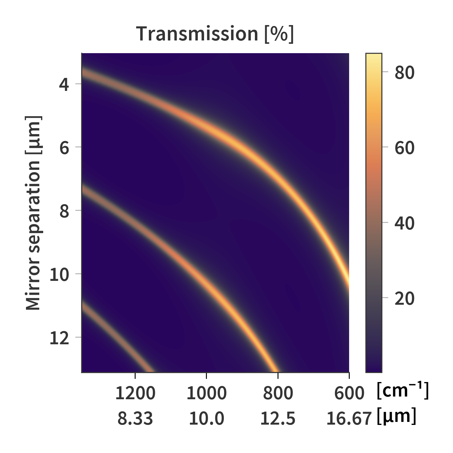
We assume that Fig. 16 as an (approximately) accurate description of the transmission through the SFPI at relevant combinations of wavelengths and mirror separations. Next, we need to account for the response of the sensor and optics. Firstly, we need to setup an expression describing the contributions to the recorded signal.
\[\begin{align} \label{eq:fpi_flux} \mathbf{\Phi} = \mathbf{T_{SFPI}}\diamond(\mathbf{t_{samp}}\circ\mathbf{m_{BB}}(T_{BB}) + (\mathbf{1} - \mathbf{t_{samp}})\circ\mathbf{m_{env}}(T_{env})) + \mathbf{R_{SFPI}} \diamond \mathbf{m_{sens}}(T_{sens}) \end{align}\]Here, $\circ$ and $\diamond$ represent element-wise and row/element-wise multiplication respectively. By row/element-wise I mean that each row of the matrix is multiplied element-wise by each element in the vector. $\mathbf{T_{SFPI}}$ and $\mathbf{R_{SFPI}}$ are the transmission and reflection matrices of the SFPI calculated using TMM. $\mathbf{t_{samp}}$ is the FTIR transmission spectrum of the sample. Since I do not have the reflectance spectra of the samples, these are estimated simply by $(\mathbf{1} - \mathbf{r_{samp}})$ (assuming the samples are loss-less). $\mathbf{m_{BB}}(T_{BB})$, $\mathbf{m_{env}}(T_{env})$, and $\mathbf{m_{sens}}(T_{sens})$ are the black body spectra of the black body behind the sample, the environmental background emission and the sensor. $T_{BB}$, $T_{env}$, and $T_{sens}$ are the temperatures of the black body, the environment, and the sensor respectively.
This expression does not include the emission spectrum of the sample itself. Also, $(\mathbf{1} - \mathbf{r_{samp}})$ is probably not a correct estimation of the sample reflectance. Furthermore, the sensor is probably not a true black body, but this works for the estimation.
$\mathbf{\Phi}$ represents the radiation incident on the sensor at different combinations of wavelengths and mirror separations for different samples. Because the microbolometer sensor measures the difference between the incident flux to its own outgoing flux, we need to subtract it from Eq. (\ref{eq:fpi_flux}) to get an expression for the recorded signal.
\[\begin{align} \label{eq:fpi_signal} \mathbf{\Delta\Phi} = \mathbf{\Phi} - \mathbf{m_{sens}}(T_{sens}) \end{align}\]Note here that the subtraction happens row/element-wise.
Before we arrive at the recorded interferogram, $\mathbf{i}$, we just need to take the dot product of $\mathbf{\Delta\Phi}$ and the sensor response, $\mathbf{x}$.
\[\begin{align} \label{eq:sensor_response_Ax=b} \mathbf{i} = \mathbf{\Delta\Phi} \mathbf{x} \end{align}\]We are now again working with an $\mathbf{Ax}=\mathbf{b}$ problem, but luckily we are only looking for $\mathbf{x}$ which probably is an easier problem (even though it is still under-determined). Since the response we are looking for cannot contain negative values, we will use the fast nonnegative least squares (FNNLS) implementation in python. To get a better representation of $\mathbf{x}$, multiple data sets are included in the calculation. This is done by concatenating all the $\mathbf{i}$’s and $\mathbf{\Delta\Phi}$’s from each sample.
\[\begin{align} \label{eq:i_concat} \begin{bmatrix} \mathbf{i_{acetone}} \\ \mathbf{i_{ammonia}}\\ \vdots\\ \mathbf{i_{toluene}}\\ \mathbf{0} \end{bmatrix} = \begin{bmatrix} \mathbf{\Delta\Phi_{acetone}} \\ \mathbf{\Delta\Phi_{ammonia}}\\ \vdots\\ \mathbf{\Delta\Phi_{toluene}}\\ \gamma_{reg}\mathbf{M}\\ \end{bmatrix} \mathbf{x} \end{align}\]Here, a regularization term is included as the last element of each ‘column vector’. The $\mathbf{0}$-vector has as many elements as the number of rows in $\mathbf{M}$, which is defined as previously. Using the FNNLS solver to solve for $\mathbf{x}$ in Eq. (\ref{eq:i_concat}) yields a sensor response presented in Fig. 17. In these estimations a number of samples have been omitted. These are for example some of the paper and plastic film samples as these exhibit severe scattering and absorptive losses which decrease the model fit.
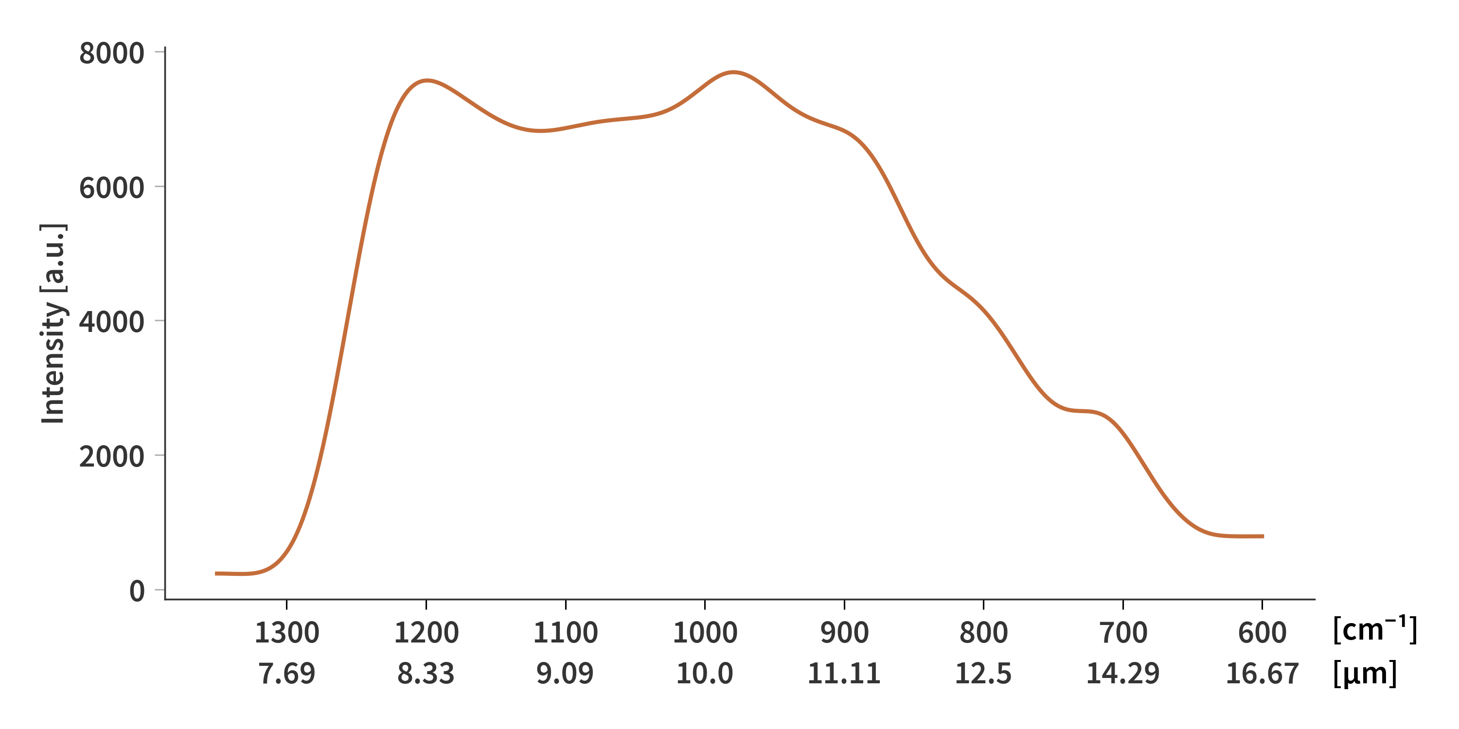
Note that he response does not go to 0 above 16 µm as expected… Not quite sure why that is. It is also slightly positive below 7.6 µm, but not quite as much. To evaluate the performance of the found response, we can plug it into Eq. (\ref{eq:sensor_response_Ax=b}). The results are quite extensive and can therefore be seen here. In this case, RRMSE is defined as
\[\begin{align} \label{eq:RRMSE} \mathrm{RRMSE} = \sqrt{\frac{\frac{1}{n} \sum_{i=1}^{n} (\hat{X}_i - X_i)^2}{\sum_{i=1}^{n} X_i^2}} \end{align}\]with $\hat{X}$ representing the predicted value and $X$ being the measured value. Relatively good agreement between predictions and measurements is achieved and even the intensities are correctly predicted. A notable improvement is the ability to include ‘negative’ contributions in the predictions. E.g. in the “air duster” and “ethylene” interferograms there are points at which the netto flux is less than when the SFPI is completely closed resulting in the interferograms dropping below 0. The combined result of the spectral response (Fig. 17) and the transmission matrix (Fig. 16) can be seen in Fig. 18.
