Estimating sensor response

Using fast nonnegative least squares (FNNLS)

I have previously had some luck with with using fast nonnegative least squares (FNNLS) to estimate the sensor response based on empirical measurements. For this I need for formulate an $\mathbf{Ax} = \mathbf{b}$ problem for the solver. It has previously been described how to set up this problem, so I will not go into much detail here_. Just know that the $\mathbf{A}$ matrix expresses the known (estimated from FTIR) net flux (incident minus emitted), $\mathbf{b}$ is the measured interferogram (without offset - we’ll discuss that later), and $\mathbf{x}$ is the sensor response we need to solve for.

\[\begin{align} \label{eq:fpi_flux} \mathbf{A} = \mathbf{T_{SFPI}}\diamond(\mathbf{t_{samp}}\circ\mathbf{m_{BB}}(T_{BB}) + \mathbf{r_{samp}}\circ\mathbf{m_{env}}(T_{env})) + \mathbf{R_{SFPI}} \diamond \mathbf{m_{sens}}(T_{sens}) - \mathbf{m_{sens}}(T_{sens}) \end{align}\]

Here, $\mathbf{t_{samp}}$, and $\mathbf{r_{samp}}$ are FTIR measurements of the sample’s transmittance and reflectance respectively. $\mathbf{T_{SFPI}}$ and $\mathbf{R_{SFPI}}$ are transmittance and reflectance estimates of the SFPI and $\mathbf{m_{subscript}}(T)$ are black body spectra at the temperature, $T$. The solution needs to be smoothness regularized, and the final system of equations for all measurements therefore becomes

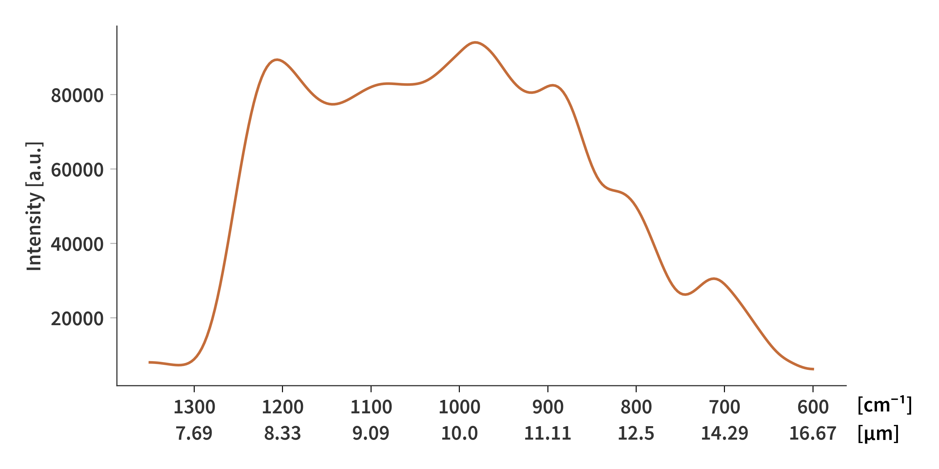
\[\begin{align} \label{eq:soe} \begin{bmatrix} \mathbf{A_{acetone}} \\ \mathbf{A_{ammonia}}\\ \vdots\\ \mathbf{A_{toluene}}\\ \gamma_{reg}\mathbf{M}\\ \end{bmatrix} \mathbf{x} = \begin{bmatrix} \mathbf{b_{acetone}} \\ \mathbf{b_{ammonia}}\\ \vdots\\ \mathbf{b_{toluene}}\\ \mathbf{0} \end{bmatrix} \end{align}\]

where $\gamma_{reg}$ is the regularization parameter, and $\mathbf{M}$ is the smoothness regularization matrix. The solution found using FNNLS is presented in Fig. 1.

Fig 1: Calculated sensor and optics response based on FNNLS solution of Eq. (\ref{eq:soe})

Finding my own gradient decent solution

But I want more control - in particular, I want to be able to account for the unknown offset, there is for every separate interferogram. But firstly, let’s see if we can’t get a similar solution to the FNNLS without the offset. The objective function is then formulated as follows

\[\begin{align} \label{eq:arg_min} \arg \min_{\mathbf{x}} ||\mathbf{b} - \mathbf{Ax}||_2^2 + \gamma_{reg}||\mathbf{Mx}||_2^2 \qquad \textrm{s.t.} \quad \mathbf{x} \geq 0 \end{align}\]

Finding the gradient with respect to $\mathbf{x}$ yields:

\[\begin{align} \label{eq:deriv_x} \nabla_\mathbf{x}\left[||\mathbf{b} - \mathbf{Ax}||_2^2 + \gamma_{reg}||\mathbf{Mx}||_2^2\right] = 2\left(\mathbf{A}^T\mathbf{Ax} - \mathbf{A}^T\mathbf{b} + \gamma_{reg}\mathbf{M}^T\mathbf{Mx}\right) \end{align}\]

The gradient decent algorithm is defined as

\[\begin{align} \label{eq:update_x} \mathbf{x} \leftarrow \mathbf{x} - 2\alpha \left(\mathbf{A}^T\mathbf{Ax} - \mathbf{A}^T\mathbf{b} + \gamma_{reg}\mathbf{M}^T\mathbf{Mx}\right), \quad \alpha = \frac{2}{||\mathbf{A}^T\mathbf{A}|| + \gamma_{reg}||\mathbf{M}^T\mathbf{M}||} \end{align}\]

Where $\alpha$ is the maximum step size as determined by the Lipschitz constant. Implemented in python, this looks like

def Ax_minus_b_w_reg(A, x, b, M, gamma, itermax):
    AtA = A.T @ A
    Atb = A.T @ b
    MtM = gamma * (M.T @ M)
    U, S_A, Vh = np.linalg.svd(AtA, full_matrices=True)
    U, S_M, Vh = np.linalg.svd(MtM, full_matrices=True)
    stepsize = 5e1/(S_A[0] + gamma * S_M[0])
   
    cost_func = []    
    v = np.copy(x)
    for i in range(itermax):
        grad_v = AtA @ v - Atb + MtM @ v
        x_old = x
        x = np.maximum(0, v-stepsize*grad_v) 
        v = x + (i/(i+3)) * (x - x_old)
        cost_func.append(0.5 * np.linalg.norm(A @ x - b)**2)
    return x, cost_func

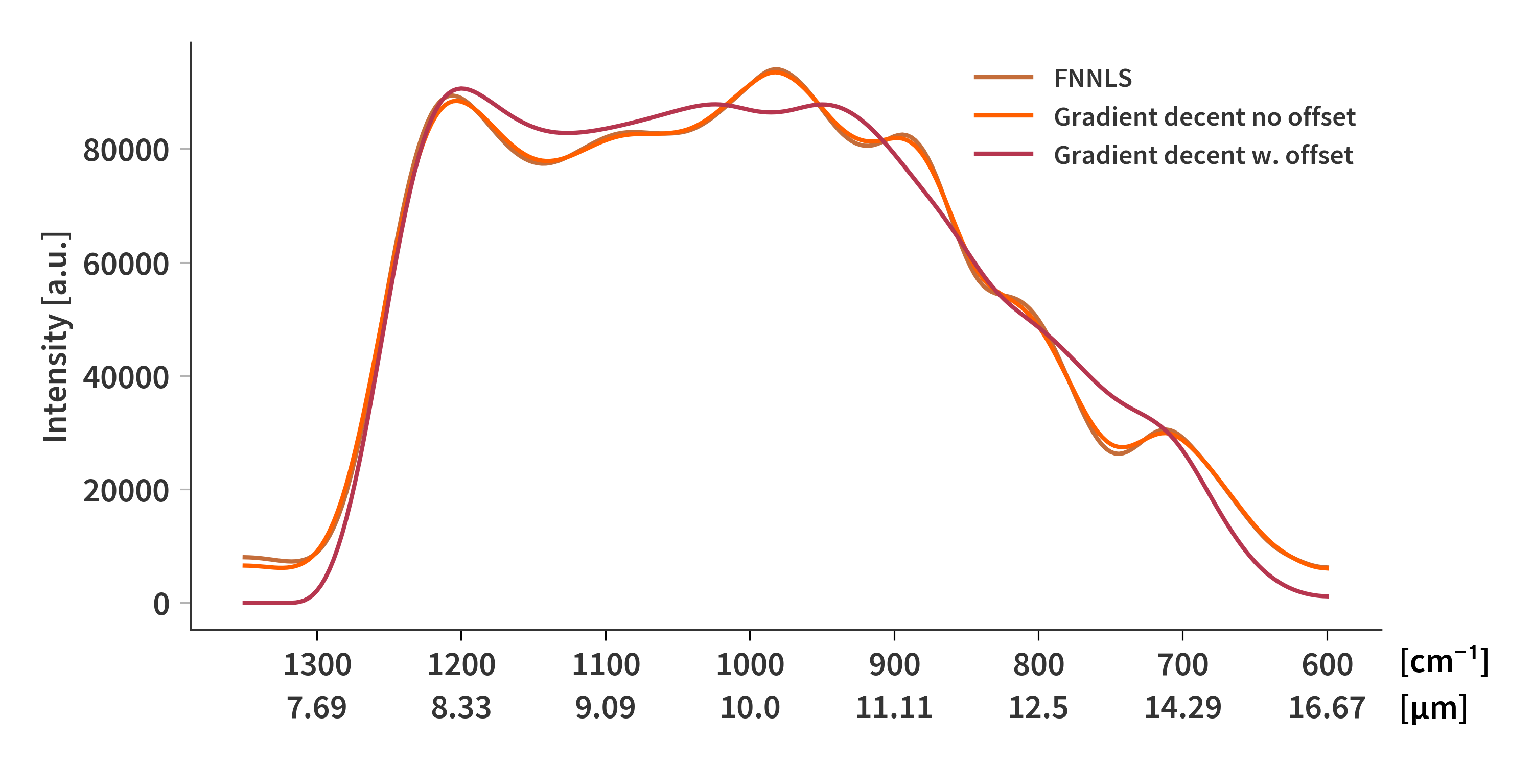
Running this 5000 times with $\gamma_{reg} = 50$ yields similar results to FNNLS as depicted in Fig. 2.

Fig 2: Sensor responses calculated using both FNNLS and gradient decent. The FNNLS prediction is performed without any offsets.

Now let’s add an offset

I want to solve for the offset separately, meaning everything else is held constant. The optimization problem then becomes

\[\begin{align} \label{eq:arg_min_offset} \arg \min_{\psi}||\mathbf{b} - \mathbf{Ax} - \psi\mathbf{1}||_2^2 = \arg \min_{\psi}||\mathbf{c} - \psi\mathbf{1}||_2^2 \end{align}\]

where $\psi$ is a constant scalar offset and $\mathbf{1}$ is a vector of 1’s with the same dimension as $\mathbf{b}$ (and $\mathbf{c}$ for that matter). The offset is mostly associated with $\mathbf{b}$ as it describes an offset to the interferograms.

The objective function can be expanded yielding

\[\begin{align} \label{eq:objective_psi} ||\mathbf{c} - \psi\mathbf{1}||_2^2 = \mathbf{c}^T\mathbf{c} - \psi\mathbf{c}^T\mathbf{1} - \psi \mathbf{1}^T\mathbf{c} + \psi^2\mathbf{1}^T\mathbf{1} = ||\mathbf{c}||_2^2 - 2\psi⟨\mathbf{c}|\mathbf{1}⟩ + \psi^2||\mathbf{1}||_2^2 \end{align}\]

which is achieved by utilizing that the matrix inner product $⟨\mathbf{A}|\mathbf{B}⟩=\textrm{Tr}(\mathbf{A}^T\mathbf{B})$ and that the trace is transpose invariant.

We notice that this is really just a quadratic function in terms of $\psi$ as we can rewrite it as

\[\begin{align} \label{eq:quadratic_psi} ||\mathbf{c}||_2^2 - 2\psi⟨\mathbf{c}|\mathbf{1}⟩ + \psi^2||\mathbf{1}||_2^2 = a_1 + a_2\psi + a_3\psi^2, \qquad a_1 = ||\mathbf{c}||_2^2, \quad a_2 = - 2⟨\mathbf{c}|\mathbf{1}⟩, \quad a_3 = ||\mathbf{1}||_2^2 \end{align}\]

$⟨\mathbf{c}|\mathbf{1}⟩$ is really just the sum of $\mathbf{c}$ and $||\mathbf{1}||_2^2$ is just the number of elements in $\mathbf{c}$. We are interested in finding the value of $\psi$ which minimizes the objective function. It is not guaranteed that the function is exactly 0 anywhere, so instead of finding roots, we simply find the derivative with respect to $\psi$ and set it equal to zero. From this we find a closed form expression for $\psi$

\[\begin{align} \label{eq:closed_psi} \psi = \frac{-a_2}{2a_3} = \frac{⟨\mathbf{c}|\mathbf{1}⟩}{||\mathbf{1}||_2^2} \end{align}\]

which is simply just the mean of $\mathbf{c}$.

But the offset is individual for each of the interferograms, so we cannot just concatenate all measurements as we have done previously. Instead, the sensor response should be calculated for all measurements (I know that’s what we have just done). Then, an offset should be calculated for each measurement separately before the sensor response is then once again calculated now including the offset in $\mathbf{b}$.

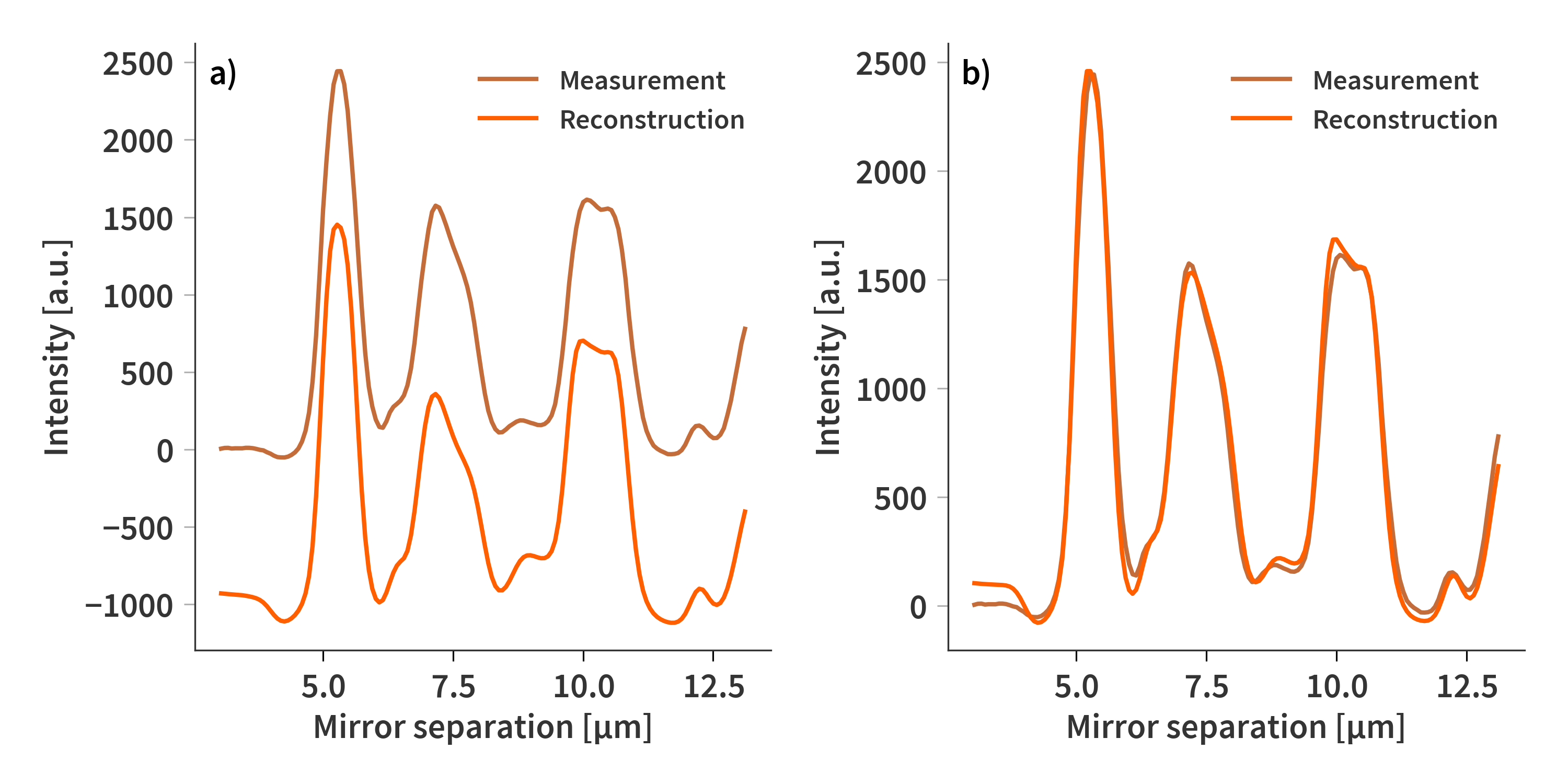
And to my own surprise, this actually appears to be working as depicted in Fig. 2 and by the reconstructions in Fig. 3.

Fig 3: Reconstructed interferograms without the offset (a) and with the offset (b).