Summary of NMF-based reconstructions
Updated:
This is going to be a broader overview of my different efforts in the attempt to reconstruct the incident spectra based on the interferograms recorded by the hyperspectral camera. The setup has been described in further detail previously_ so here is just a very short introduction of the problem in terms of an $\mathbf{AX}= \mathbf{B}$ problem. The system matrix, $\mathbf{A}$ describes the transmission through the Fabry-Pérot interferometer at different combinations of wavelengths and mirror separations. A sensor response has been fitted an multiplied with each row of $\mathbf{A}$ (each row represent the transmission spectrum in terms of wavelengths/wavenumbers at a specific mirror separation). Each column of $\mathbf{X}$ contains the incident spectrum of the sample. This spectrum is a combination of the light source being transmitted through the material sample along with a reflection component coming from the environment. Both the transmission and reflection measurements are obtained by FTIR spectroscopy (not ATR, but two separate measurements). Finally, $\mathbf{B}$ contains the measured interferograms from the camera. However it is not the raw measurements, but a term including the reflection of imaging sensor off the backside of the scanning Fabry-Pérot interferometer (SFPI) has also been included.
Comparison between theoretical and fit system matrix
The system matrix $\mathbf{A}$ is calculated based on the Transfer Matrix Method (TMM). Just as a kind of sanity check, lets see of it is possible to estimate $\mathbf{A}$ based on the measurement data alone and get a similar result. We can pretty easily treat this as an NMF problem where we are only fitting in terms of the “dictionary” - in this case the system matrix. The only thin is that we will need some of the usual smoothness regularization - and this is both along the rows and the columns. The minimization problem then becomes
\[\begin{align} \label{eq:min_prob_A} \arg \min_{\mathbf{A}}\frac{1}{2}||\mathbf{AX} - \mathbf{B}||_F^2 + \frac{\lambda}{2}||\mathbf{MA}||_F^2 + \frac{\gamma}{2}||\mathbf{NA}^T||_F^2 \quad \textrm{s.t.} \quad \mathbf{A} \geq \mathbf{0} \end{align}\]Here, $\mathbf{M}$ and $\mathbf{N}$ are square matrices containing $2$’s along their diagonal and $-1$ on the off diagonals. $\lambda$ and $\gamma$ are the regularization parameters controlling the regularization along the columns and rows respectively. The update step for the gradient decent algorithm then becomes
\[\begin{align} \label{eq:A_GD} \mathbf{A}^+ = \mathbf{A} - \frac{\mathbf{AXX}^T - \mathbf{BX}^T + \lambda\mathbf{M}^T\mathbf{MA} + \gamma\mathbf{WN}^T\mathbf{N}}{||\mathbf{XX}^T||_F + \lambda||\mathbf{M}^T\mathbf{M}||_F + \gamma||\mathbf{N}^T\mathbf{N}||_F} \end{align}\]The animation in Fig. 1 show a comparison between the result of the gradient decent algorithm and the TMM result. The percentages indicate the blending relationship between the two. Though the NMF solution is more noisy than the TMM, the location of the transmission bands are the same indicating that TMM is a good estimate of the system matrix. The TMM based system matrix will therefore be used as $\mathbf{A}$ for the remaining part of this post.
Reconstruction of X from A and B
The overall goal of this is to reconstruct the wavelength/wavenumber dependent spectra based on the interferograms. The coming sections document some of the ways I have been trying to achieve an estimate of $\mathbf{X}$.
Solve $\mathbf{AX} - \mathbf{B}$ for $\mathbf{X}$ using NMF
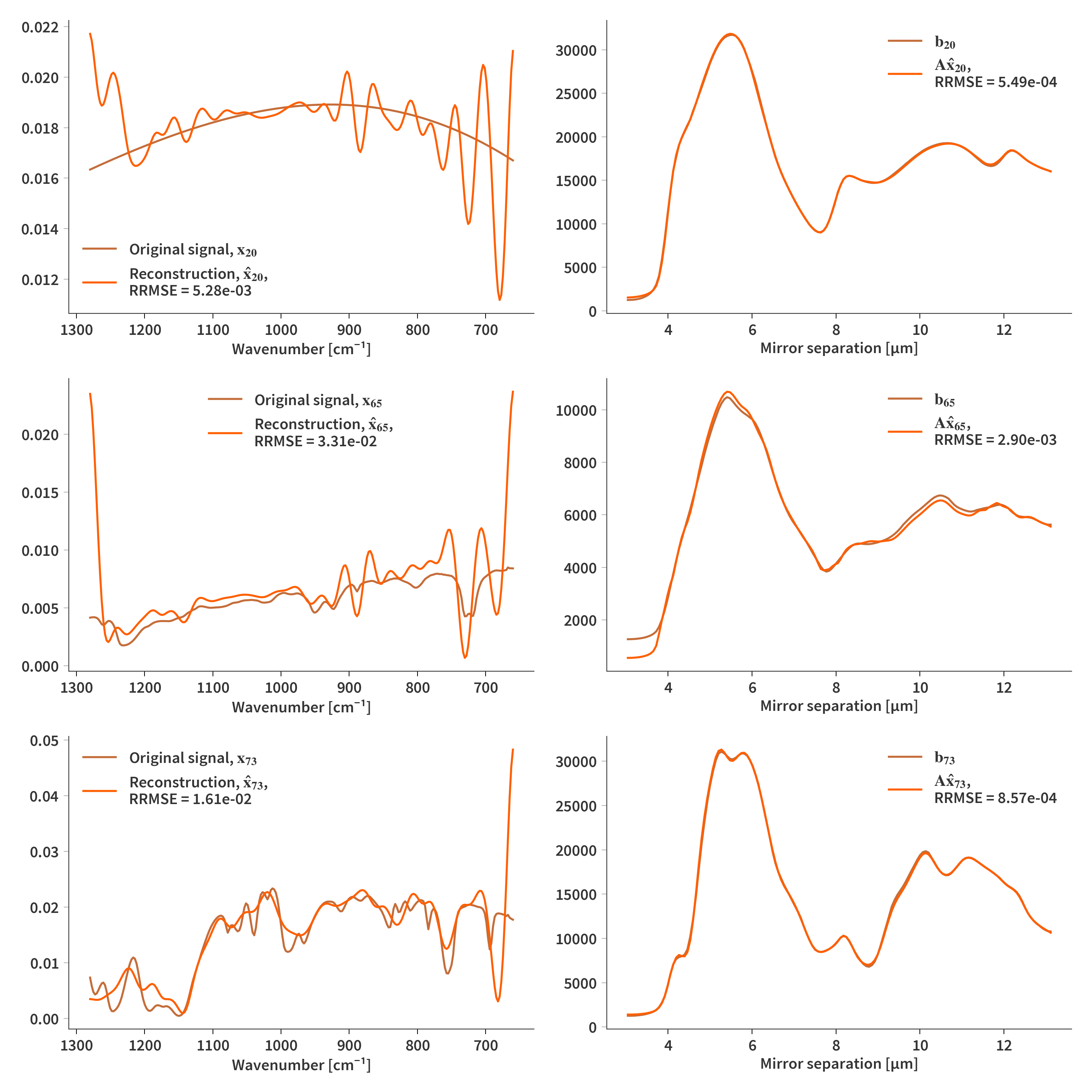
The most obvious starting step would be to use Eq. (\ref{eq:min_prob_A}) and minimize $\mathbf{X}$ instead of $\mathbf{A}$. The gradient decent step then becomes
\[\begin{align} \label{eq:X_GD} \mathbf{X}^+ = \mathbf{X} - \frac{\mathbf{A}^T\mathbf{AX} - \mathbf{A}^T\mathbf{B} + \lambda\mathbf{M}^T\mathbf{MX}}{||\mathbf{A}^T\mathbf{A}||_F + \lambda||\mathbf{M}^T\mathbf{M}||_F} \end{align}\]Notice that the smoothness regularization is now limited to be along each column, since the measurements represented in the columns of $\mathbf{X}$ are uncorrelated. A couple of results are presented in Fig. 2.
Using dictionaries to aid in reconstruction
It may seem that the solution space has to be limited in order to get closer to a “believable” spectrum. We are therefore going to factor the signals into a superposition of basis functions. The original problem can then be written in the form
\[\begin{align} \label{eq:dictionary_learning} \arg \min_{\mathbf{H}}\frac{1}{2}||\mathbf{AW\hat{X}} - \mathbf{B}||_F^2 \end{align}\]where $\mathbf{W}$ is referred to as the dictionary and $\mathbf{\hat{X}}$ is the coefficients used to reconstruct the original spectrum $\mathbf{X} = \mathbf{W\hat{X}}$. The columns of $\mathbf{W}$ are sometimes referred to as “atoms” and represent the basis functions we want to combine to estimate $\mathbf{X}$. It is possible to also fit $\mathbf{W}$, but in most (if not all) of the following examples, $\mathbf{W}$ will be predefined in order to make sure that the atoms remain physical and are not trained to recognize features which lie outside the capabilities of the camera (overfit).
Gaussian dictionary
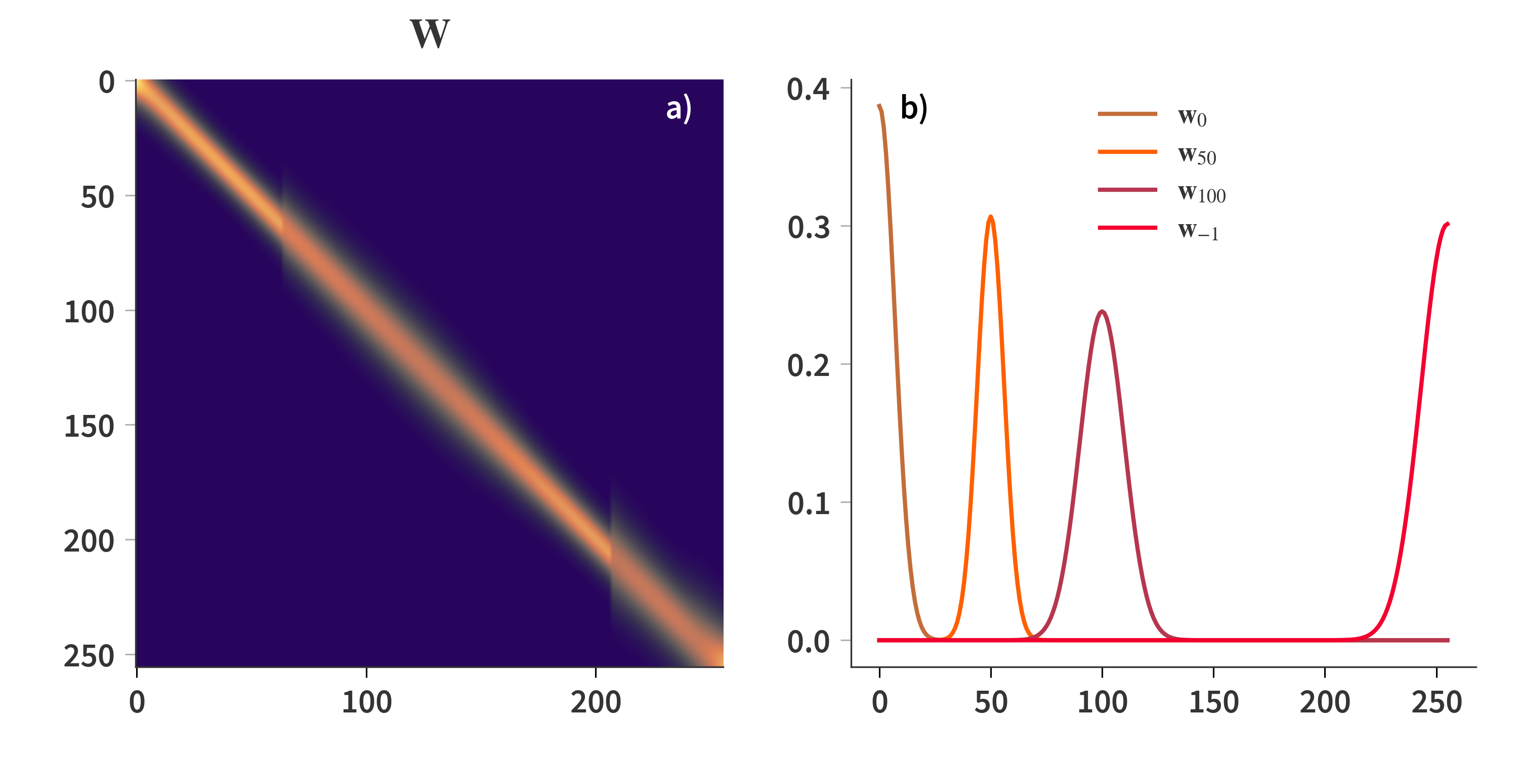
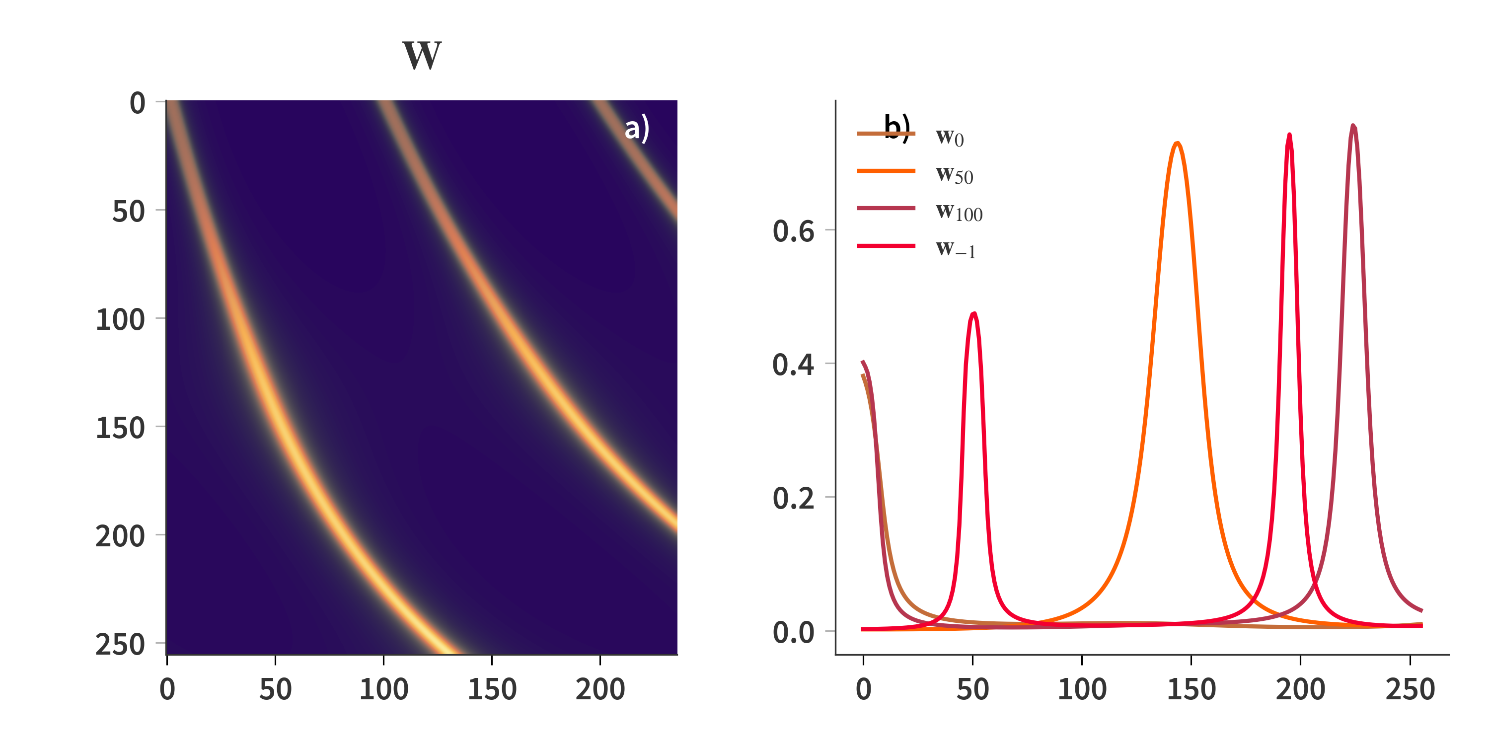
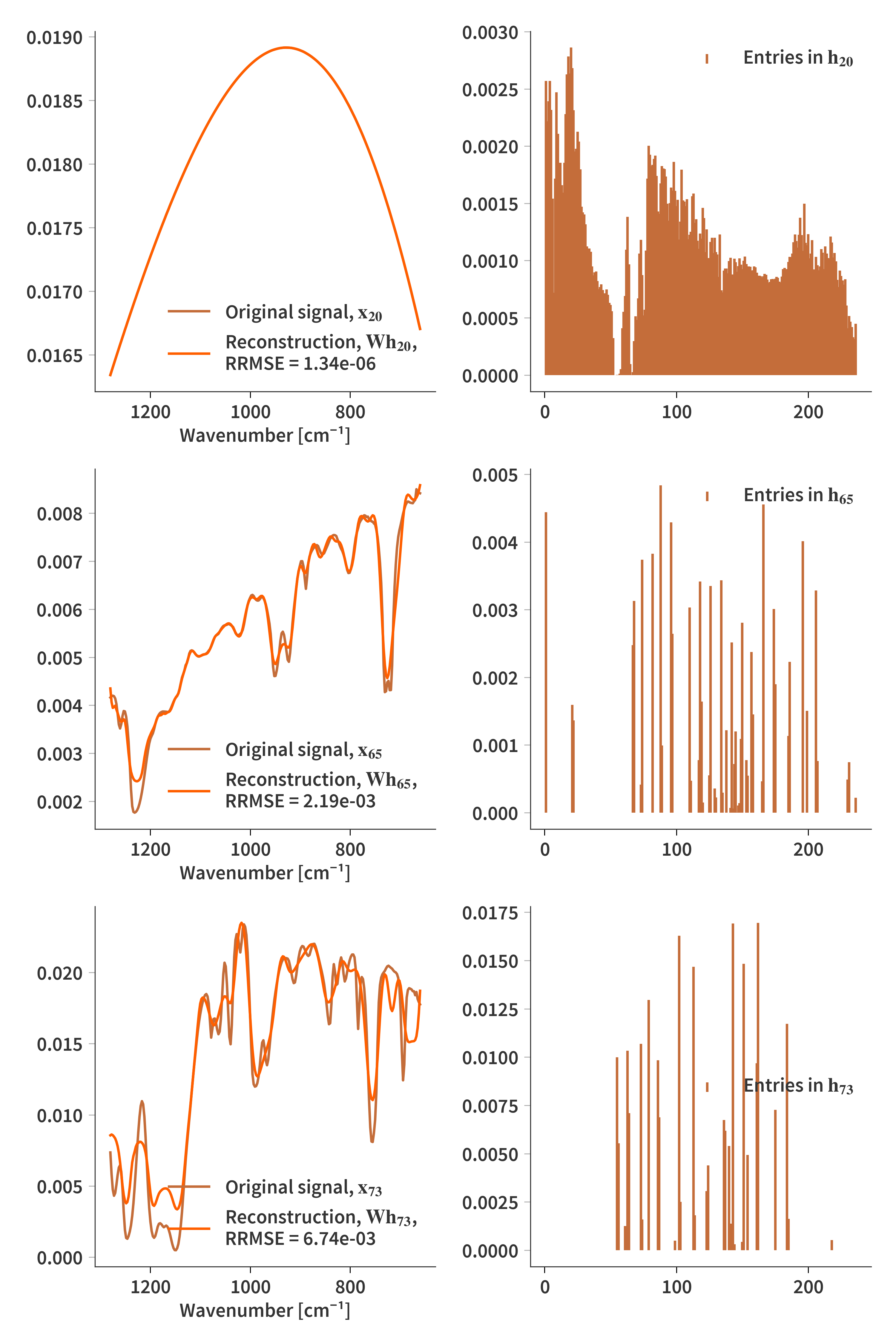
This section will document the results of using a dictionary consisting of Gaussians. A theoretically best resolution of the Fabry-Pérot is determined for each wavelength, and a Gaussian profile is constructed. That means that each column of $\mathbf{W}$ contains a single Gaussian at a given wavelength with a FWHM corresponding to the determined resolution. There are there regions of the dictionary which is depicted in Fig. 3, which correspond to the first three transmission orders of the SFPI. The lower orders have lower (worse) resolution which is why the Gaussians in this part is broader.
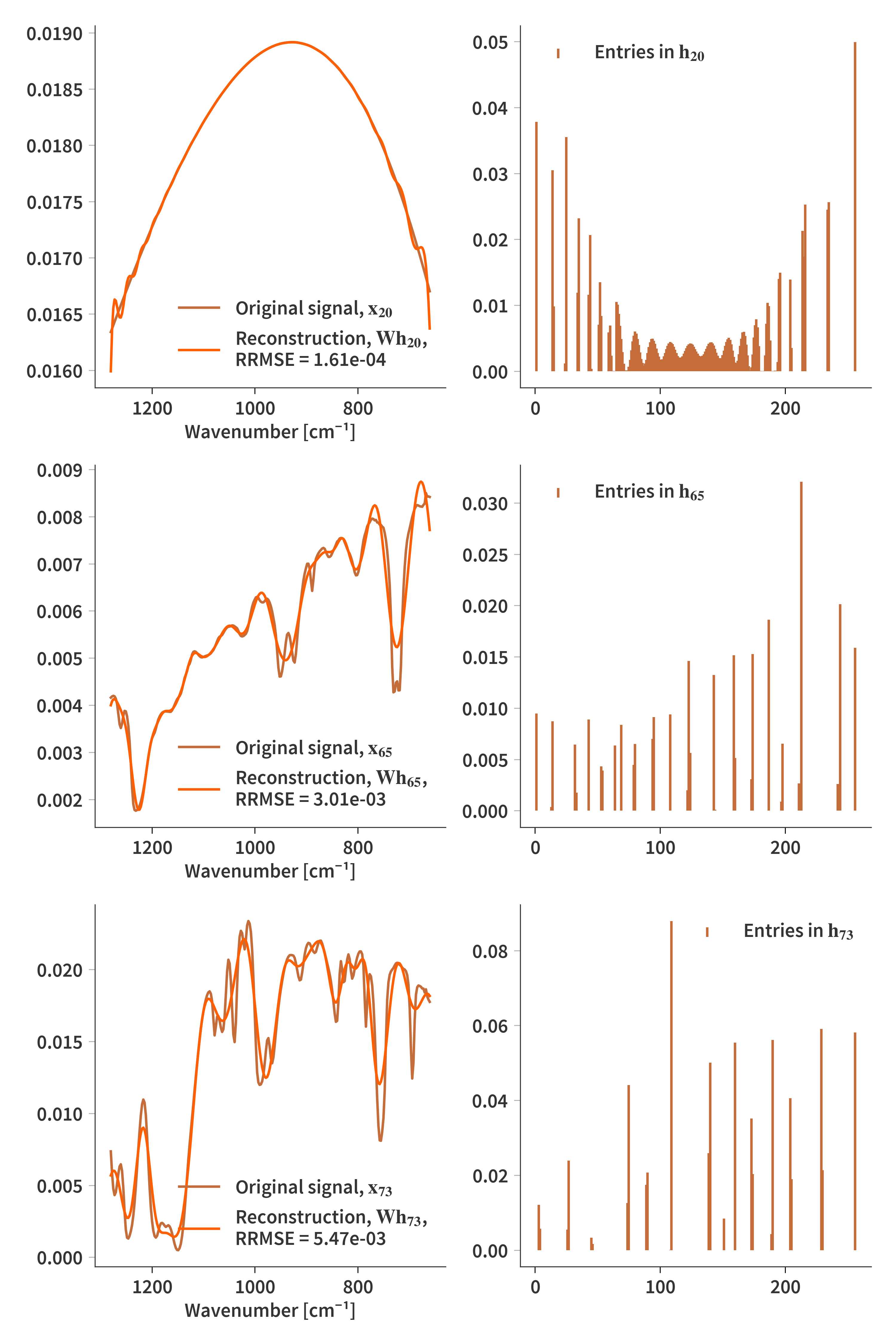
Firstly we shall see if we can even reconstruct the “TRUE” spectra using this dictionary. Therefore we are going to solve the following problem
\[\begin{align} \label{eq:NMF_H} \arg \min_{\mathbf{H}}\frac{1}{2}||\mathbf{WH} - \mathbf{X}||_F^2 \end{align}\]After gradient decent we get the following result for the reconstructions $\mathbf{WH}$
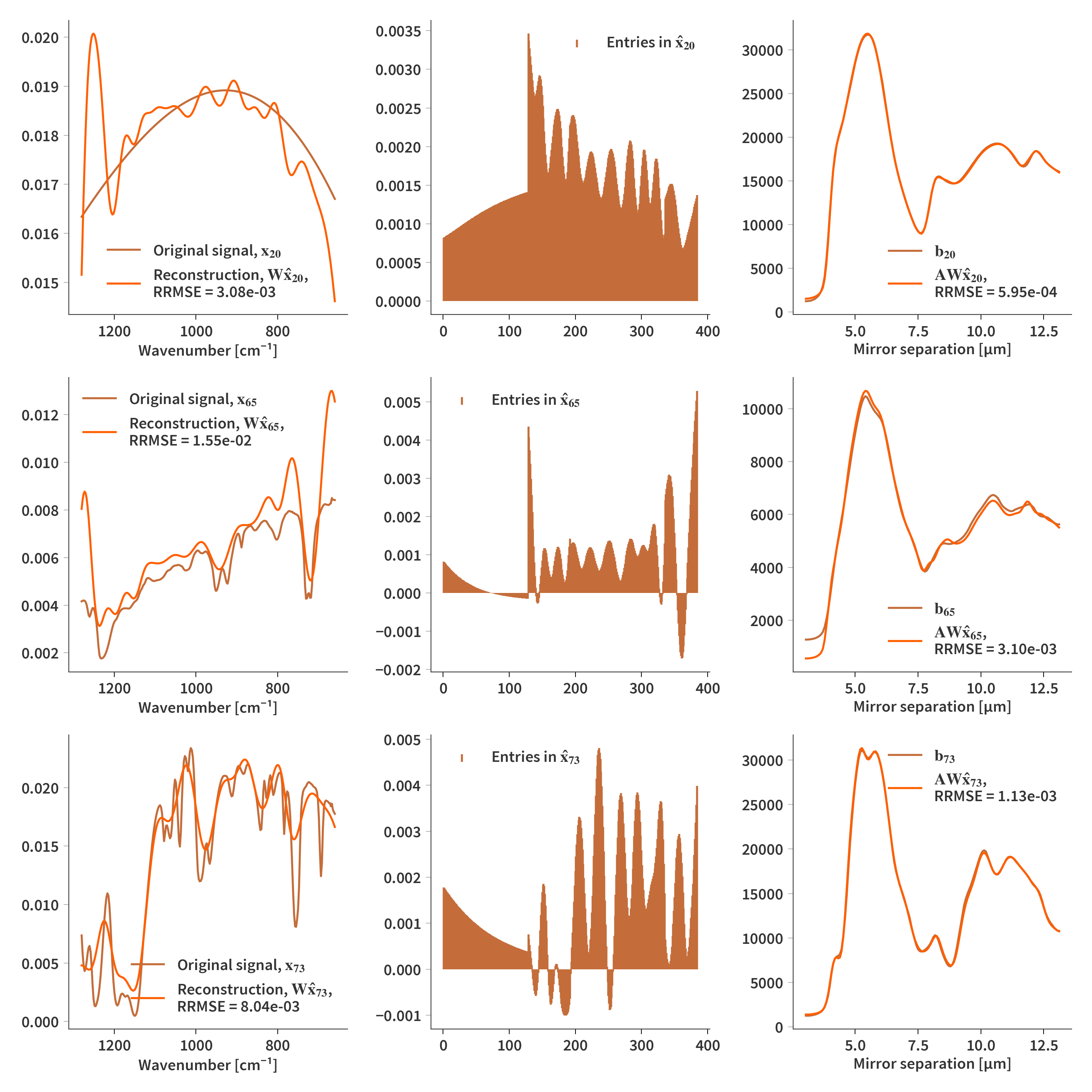
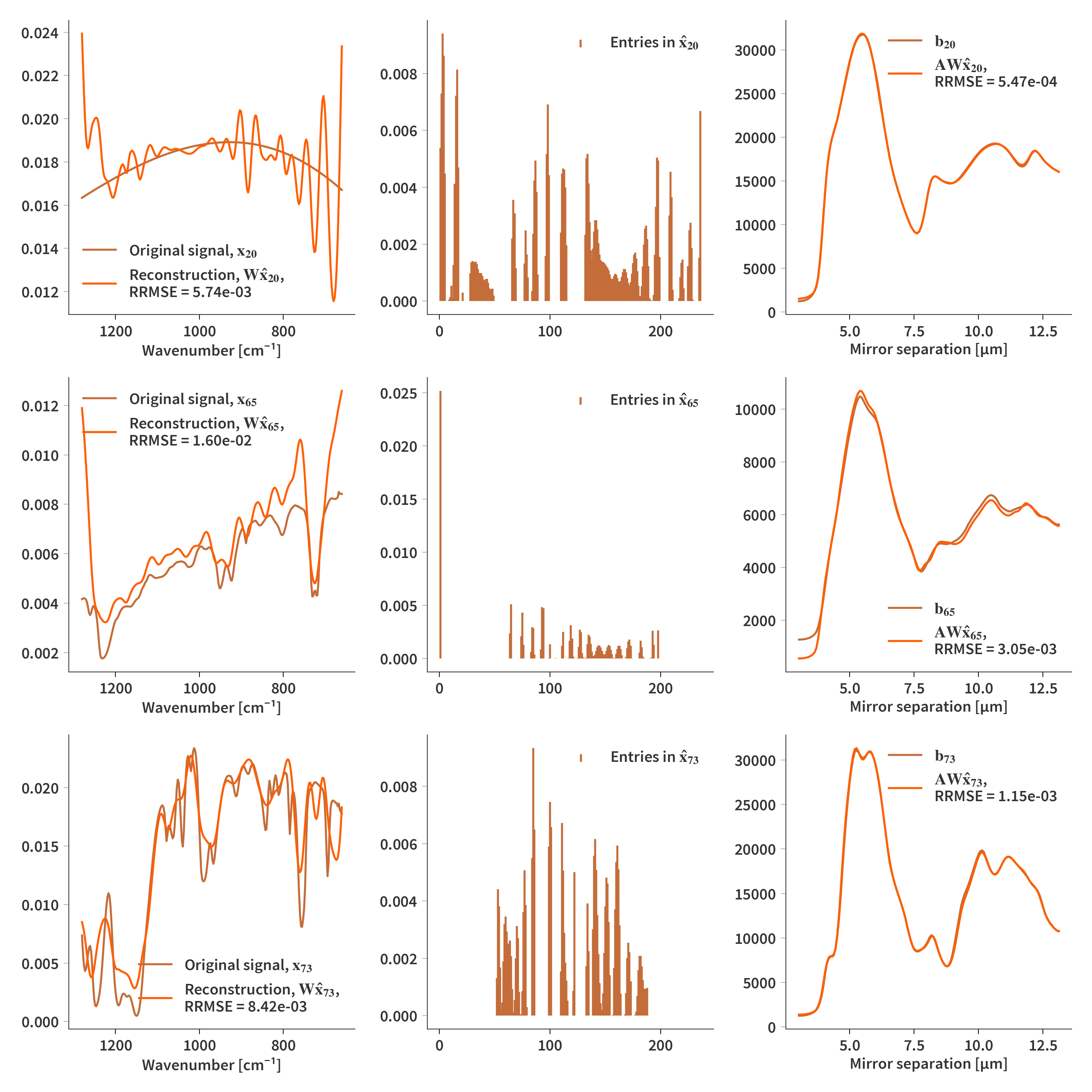
Now we can look at solving the problem stated in Eq. (\ref{eq:dictionary_learning}). We are going to solve it using NMF where we combine the system matrix and the dictionary into a new variable: $\mathbf{\hat{A}} = \mathbf{AW}$. At first we are not going to add any further regularization - only constraint is that $\mathbf{H}$ must be nonnegative. The final estimate of the spectrum is then simply $\mathbf{\hat{X}} = \mathbf{WH}$. Using this we get reconstructions as depicted in Fig. 5
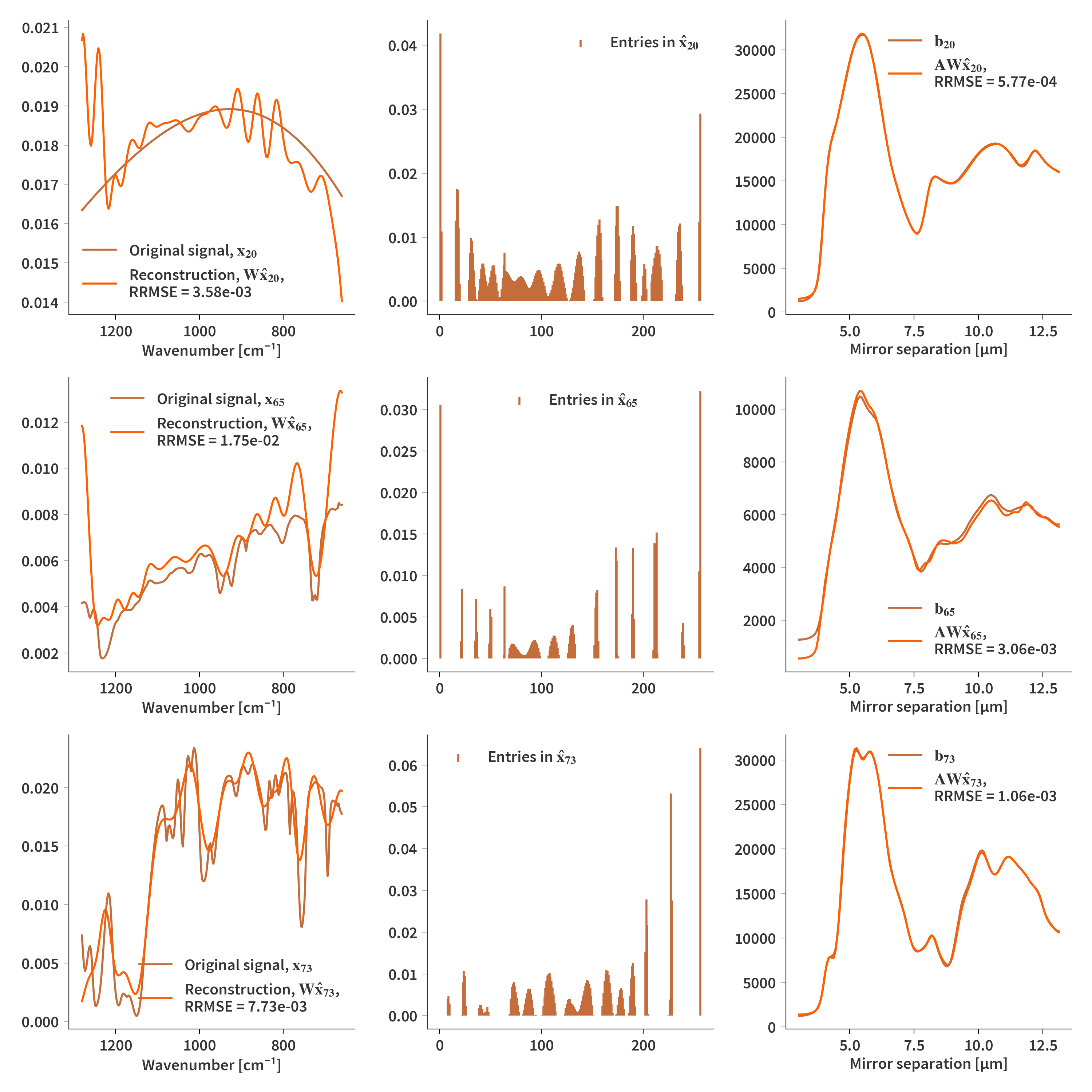
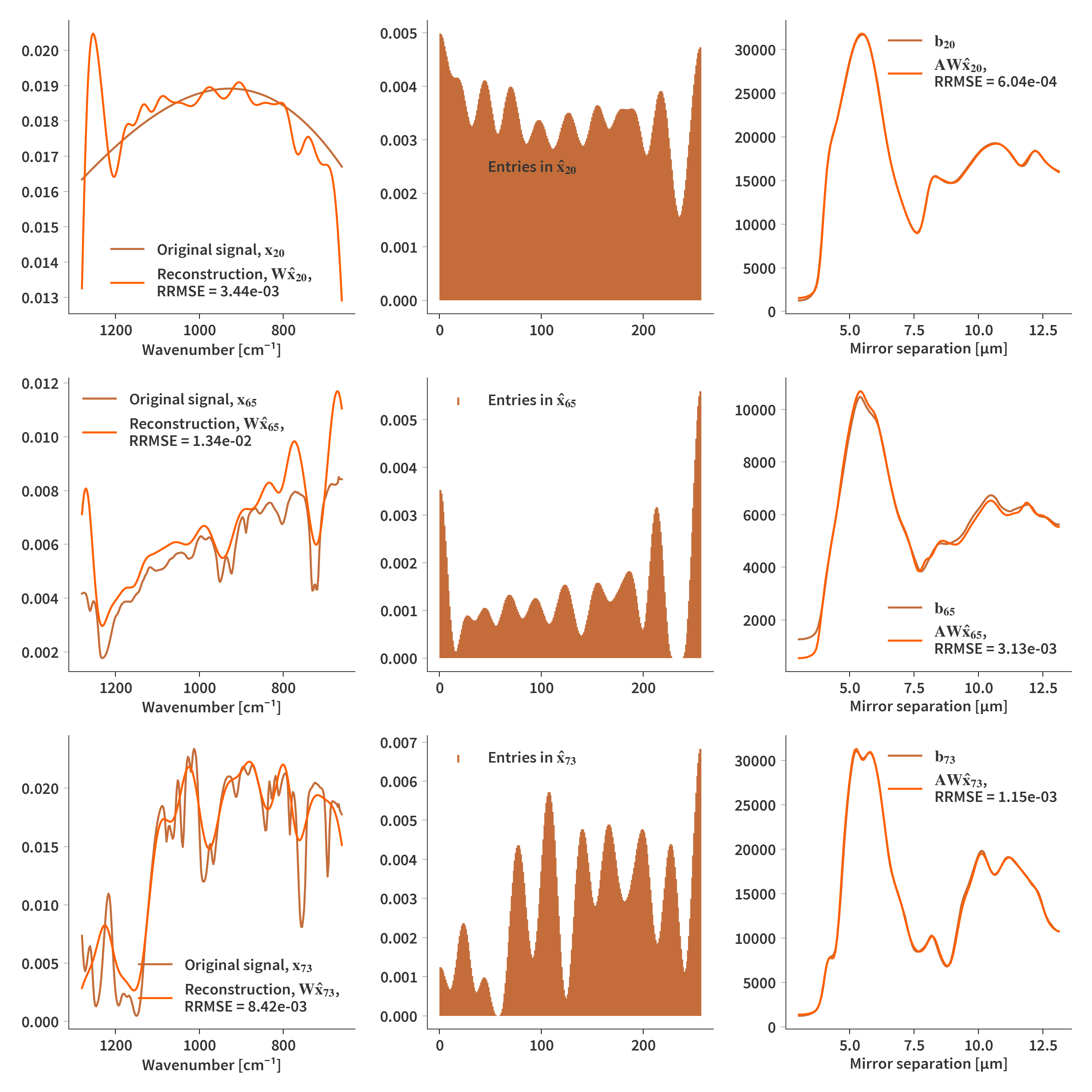
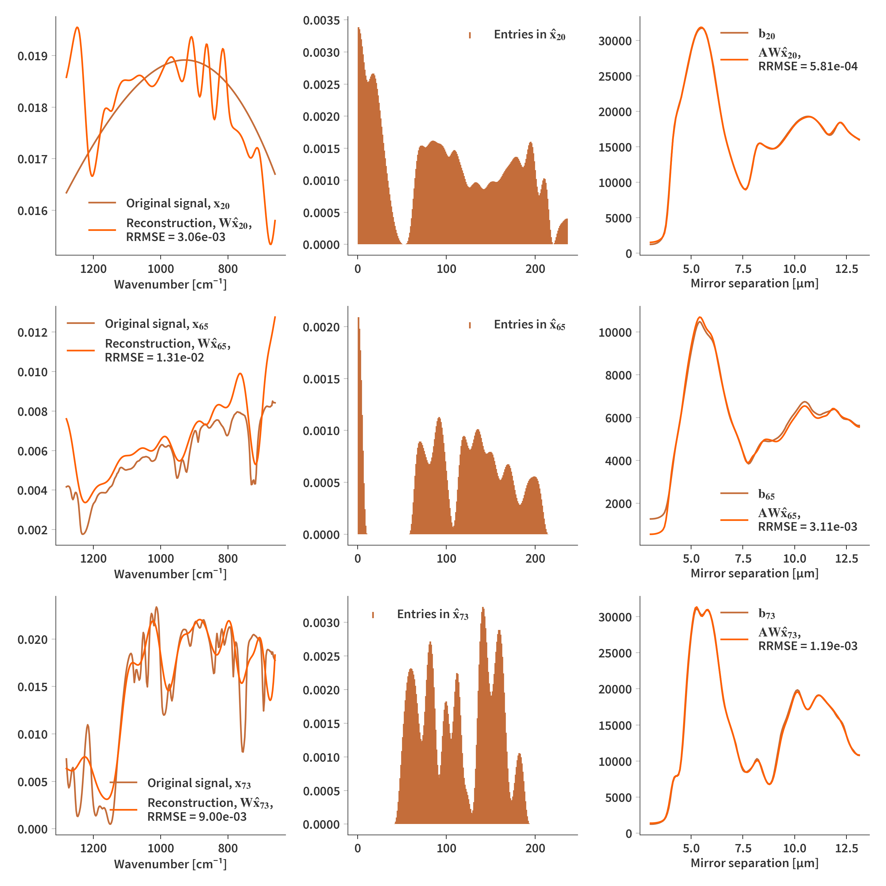
Since the atoms of the dictionary are correlated, we try to add smoothness regularization to the columns of $\mathbf{H}$ (but $\lambda$ needs to be on the order of $10^{12}$). This yields the result presented in Fig. 6
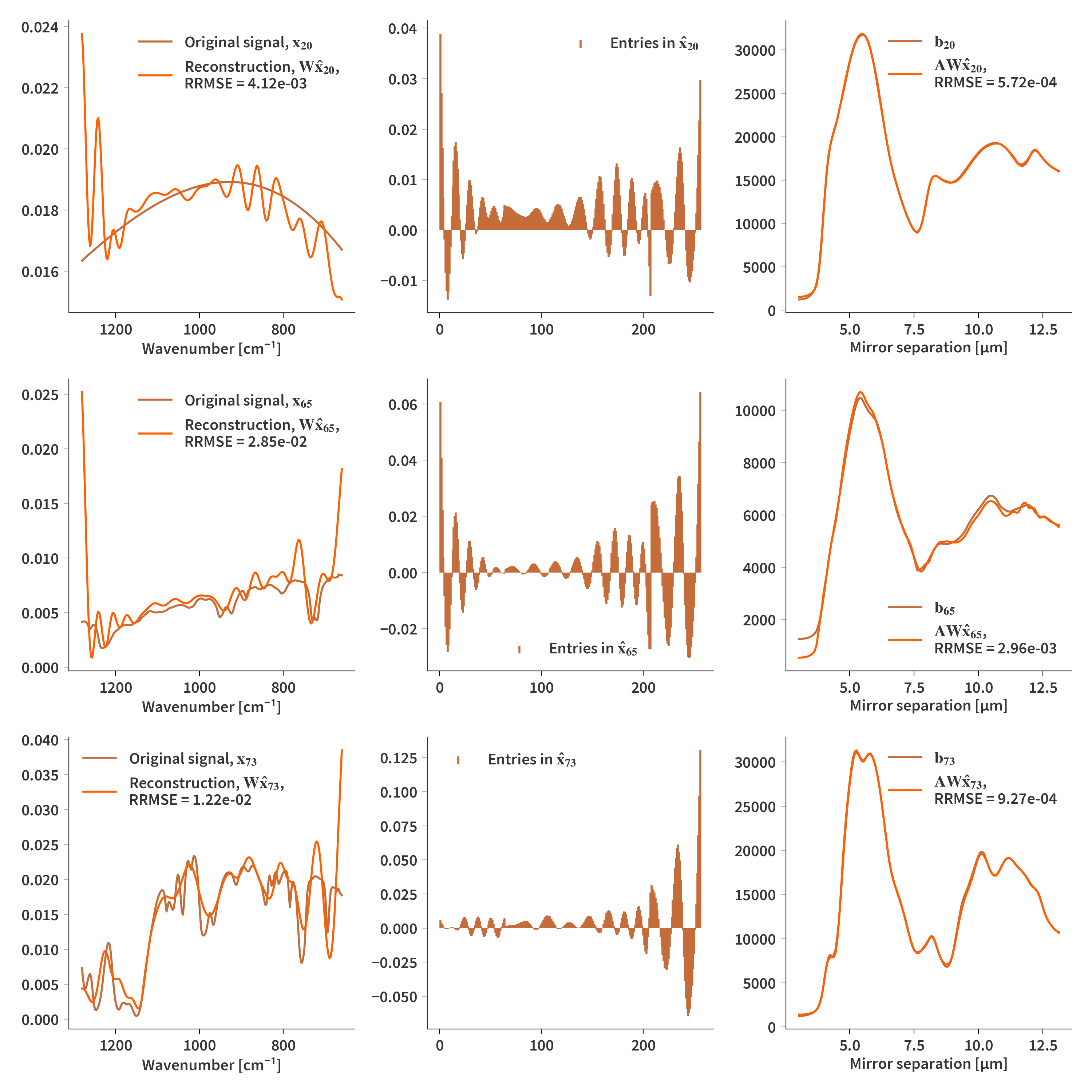
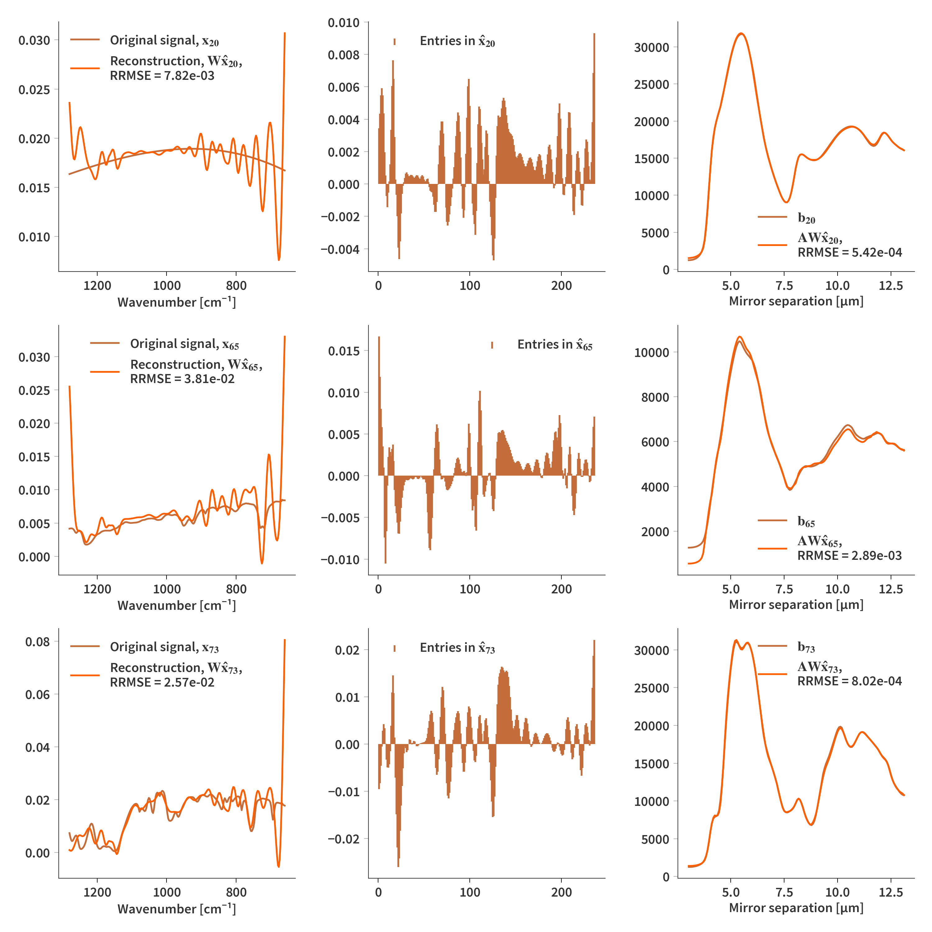
Finally we are going to see what will happen if we also relieve the nonnegativity constraint of NMF. Fig. 7 depicts the result with no regularization or constraint on $\mathbf{H}$ of any kind
Using TMM to determine dictionary
In this section we are going to use a different dictionary, which is based on the transmission of the FPI at various mirror separation. That means that each atom of the dictionary represents the transmission of the SFPI at a given mirror separation. Note that unlike for the system matrix, $\mathbf{A}$, the spectral response of the sensor and optics have not been included. This is purely the transmission of the SFPI itself and is depicted in Fig. 8.
Let’s first see how this dictionary fares for reconstructing the ground truth spectra
Now let’s look at real reconstructions
The same correlation argument between the atoms can be used here, and we will therefore see, what this does to the reconstructions.
Again, we will see, what happens if there are no constraints and no regularization
Compound constraint on $\mathbf{WH}$
It may be beneficial to allow the coefficients to be negative if what we are trying to model is a small dip in a broader spectrum. Say the spectrum is a black body curve and there is only a single dip at a given wavelength. If we are working with a Gaussian dictionary and only allow positive coefficients in $\mathbf{H}$, it will require many non-zero elements. However, if we are able to describe the broader spectrum with just a couple of coefficients and then afterwards subtract the dip, we can do with much fewer coefficients. Still, we require the reconstruction to be nonnegative as described below. \(\begin{align} \label{eq:min_prob} \arg \min_{\mathbf{H}}\frac{1}{2}||\mathbf{WH} - \mathbf{X}||_F^2 \quad \textrm{s.t. } \mathbf{WH} \geq \mathbf{0} \end{align}\)
In other words, we want to find a linear combination of the atoms in the dictionary $\mathbf{W}$ which best describes $\mathbf{X}$… So far nothing new. But now we have a compound constraint where we allow entries in $\mathbf{H}$ to be negative as long as the inner product with $\mathbf{W}$ remains nonnegative - that is because we know the signal we are trying to reconstruct (columns of $\mathbf{X}$) is nonnegative.
We already know that the gradient decent step of Eq. (\ref{eq:min_prob}) without the constraint is
\[\begin{align} \label{eq:H_step} \mathbf{H}^{+} = \mathbf{H} - \frac{\mathbf{W}^T\mathbf{WH} - \mathbf{W}^T\mathbf{X}}{||\mathbf{W}^T\mathbf{W}||_F} \end{align}\]Now to implement the constraint, we are going to solve the following problem
\[\begin{align} \label{eq:min_prob_Y,U} &\arg \min_{\mathbf{Y},\mathbf{U}}\frac{1}{2}||\mathbf{Y} - \mathbf{H}^+||_F^2 \quad \textrm{s.t. } \mathbf{WY} \geq \mathbf{0}, \quad \mathbf{WY}= \mathbf{U} \\ \Rightarrow&\arg \min_{\mathbf{Y},\mathbf{U}} \frac{1}{2}||\mathbf{Y} - \mathbf{H}^+||_F^2 + \frac{\lambda}{2}||\mathbf{WY} - \mathbf{U}||_F^2 \quad \textrm{s.t. } \mathbf{U} \geq \mathbf{0} \end{align}\]This is then split up in a $\mathbf{Y}$ and a $\mathbf{U}$ update step. It turns out that it is possible to get a closed form solution for $\mathbf{Y}$. The derivative of the first term is
\[\begin{align} \label{eq:first_deriv_Y} \frac{\partial}{\partial \mathbf{Y}} \frac{1}{2}||\mathbf{Y} - \mathbf{H}^+||_F^2 = \frac{1}{2}\frac{\partial}{\partial \mathbf{Y}} \textrm{Tr}\{\mathbf{Y}^T\mathbf{Y} - \mathbf{Y}^T\mathbf{H^+} - \mathbf{H^+}^T\mathbf{Y} + \mathbf{H^+}^T\mathbf{H^+}\} = \mathbf{Y} - \mathbf{H^+} \end{align}\]and for the second term
\[\begin{align} \label{eq:second_deriv_Y} \frac{\partial}{\partial \mathbf{Y}} \frac{\lambda}{2}||\mathbf{WY} - \mathbf{U}||_F^2 = \lambda\left(\mathbf{W}^T\mathbf{WY} - \mathbf{W}^T\mathbf{U} \right) \end{align}\]Combining Eq. (\ref{eq:first_deriv_Y}) and (\ref{eq:second_deriv_Y}) and putting the expression equation allows us to arrive at the closed form solution
\[\begin{align} \label{eq:Y_closed_form} &\mathbf{Y} - \mathbf{H^+} + \lambda\left(\mathbf{W}^T\mathbf{WY} - \mathbf{W}^T\mathbf{U} \right) = \mathbf{0} \\ \Rightarrow & \left(\mathbf{I} + \lambda \mathbf{W}^T\mathbf{W}\right)\mathbf{Y} = \mathbf{H^+} + \lambda\mathbf{W}^T\mathbf{U} \\ \Rightarrow & \mathbf{Y} = \left(\mathbf{I} + \lambda \mathbf{W}^T\mathbf{W}\right)^{-1} \left(\mathbf{H^+} + \lambda\mathbf{W}^T\mathbf{U} \right) \end{align}\]The $\mathbf{U}$ step is also straight forward
\[\begin{align} \label{eq:deriv_U} \frac{\partial}{\partial \mathbf{U}} \frac{\lambda}{2}||\mathbf{WY} - \mathbf{U}||_F^2 &= \frac{\lambda}{2}\frac{\partial}{\partial \mathbf{U}} \textrm{Tr}\{\mathbf{Y}^T\mathbf{W}^T\mathbf{WY} - \mathbf{Y}^T\mathbf{W}^T\mathbf{U} - \mathbf{U}^T\mathbf{WY} + \mathbf{U}^T\mathbf{U}\} \\ & = \lambda \left(\mathbf{U} - \mathbf{WY} \right) \end{align}\]Rearranging and implementing the nonnegativity constraint yield the following closed form solution for $\mathbf{Y}$
\[\begin{align} \label{eq:U_closed_form} \mathbf{U} = \textrm{max}\{\mathbf{0}, \mathbf{WY}\} \end{align}\]The complete update scheme of the gradient decent algorithm can be seen implemented in pseudo code below
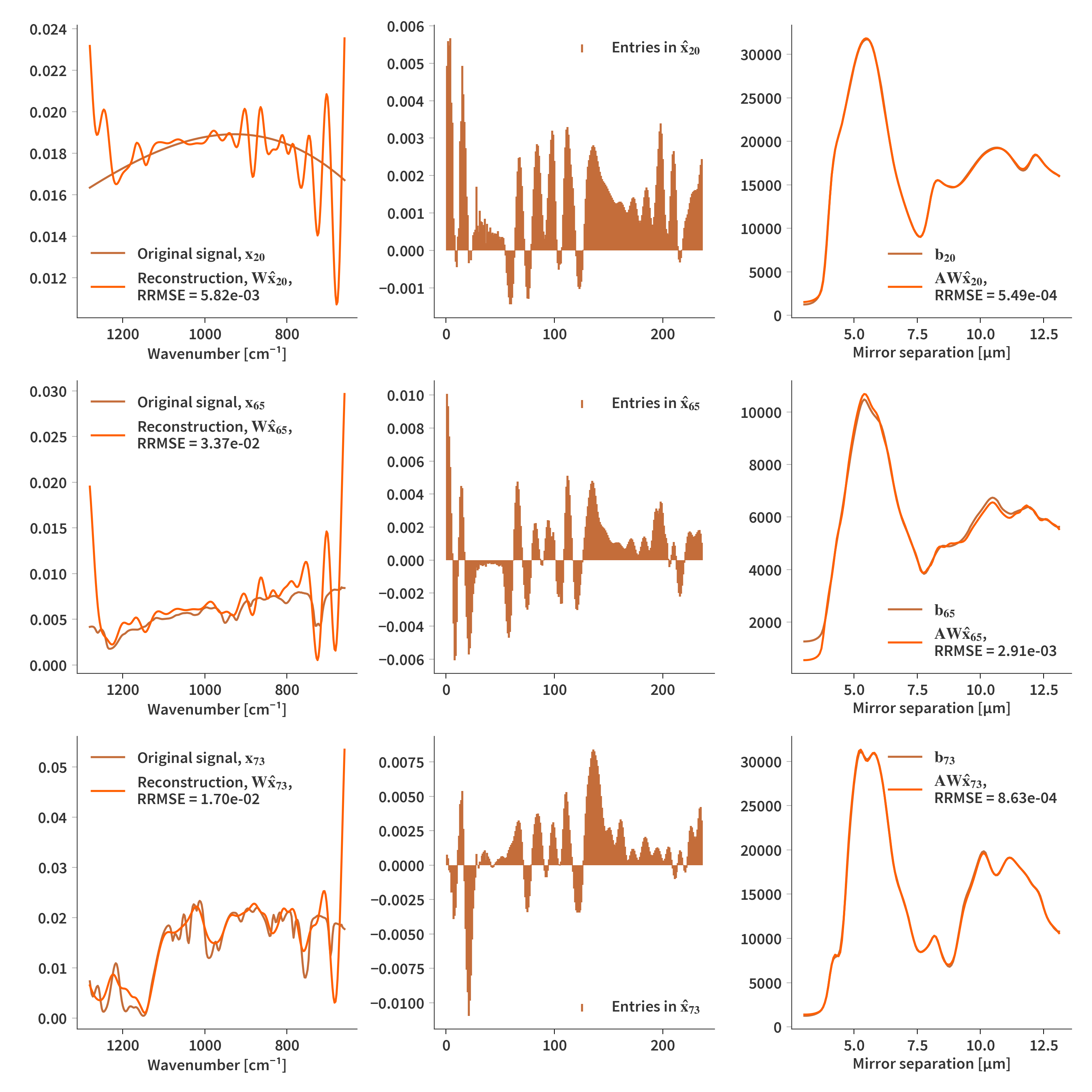
\[\begin{align} \label{eq:for_loop} & 1 \quad \textrm{for } i \in \{1 \dots Z_n\} \textrm{ do} \nonumber \\[1.0em] & 2 \quad\quad\quad \mathbf{H}^+ = \mathbf{H} - \frac{\mathbf{W}^T\mathbf{WH} - \mathbf{W}^T\mathbf{X}}{||\mathbf{W}^T\mathbf{W}||_F} \nonumber \\[1.0em] & 3 \quad\quad\quad \mathbf{U} = \mathbf{WH}^+ \nonumber \\[1.0em] & 4 \quad\quad\quad \textrm{for } j \in \{1, 2\} \textrm{ do} \nonumber \\[1.0em] & 5 \quad\quad\quad\quad\quad \mathbf{Y} = \left(\mathbf{I} + \lambda \mathbf{W}^T\mathbf{W}\right)^{-1} \left(\mathbf{H^+} + \lambda\mathbf{W}^T\mathbf{U} \right) \nonumber \\[1.0em] & 6 \quad\quad\quad\quad\quad \mathbf{U} = \textrm{max}\{\mathbf{0}, \mathbf{WY}\} \nonumber \\[1.0em] & 7 \quad\quad\quad \mathbf{H} = \mathbf{Y} \nonumber \end{align}\]Firstly we will see how it works on ground truth spectra. Here $\lambda = 10$
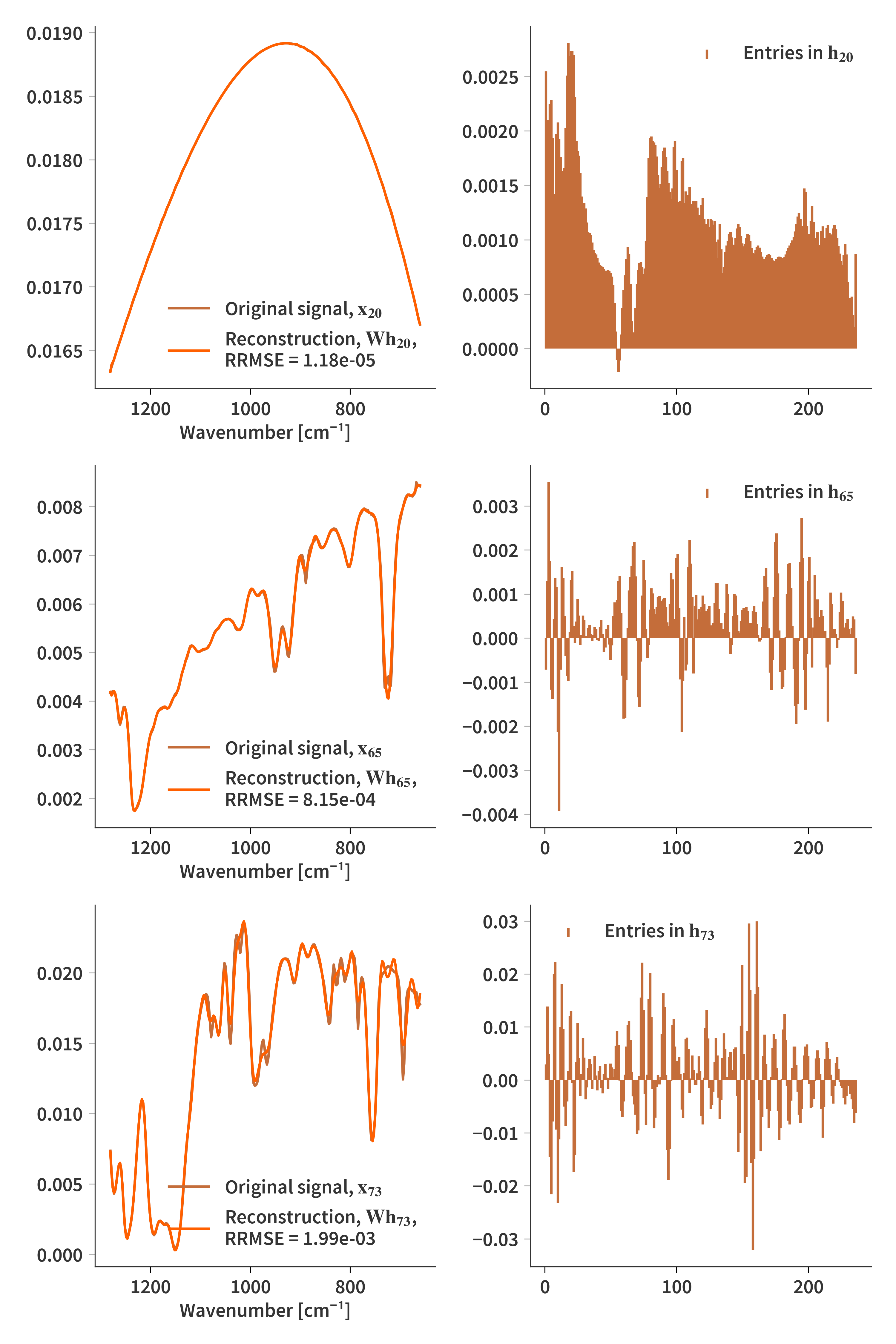
And then on reconstructions. Here $\lambda = 10^{-9}$
Black bodies in Gaussian dictionary
The real reason I wanted to try this form of regulation was to include black body radiation curves in the dictionary. A number of black body curves at different temperatures are added to the Gaussian dictionary as depicted in Fig. 15.
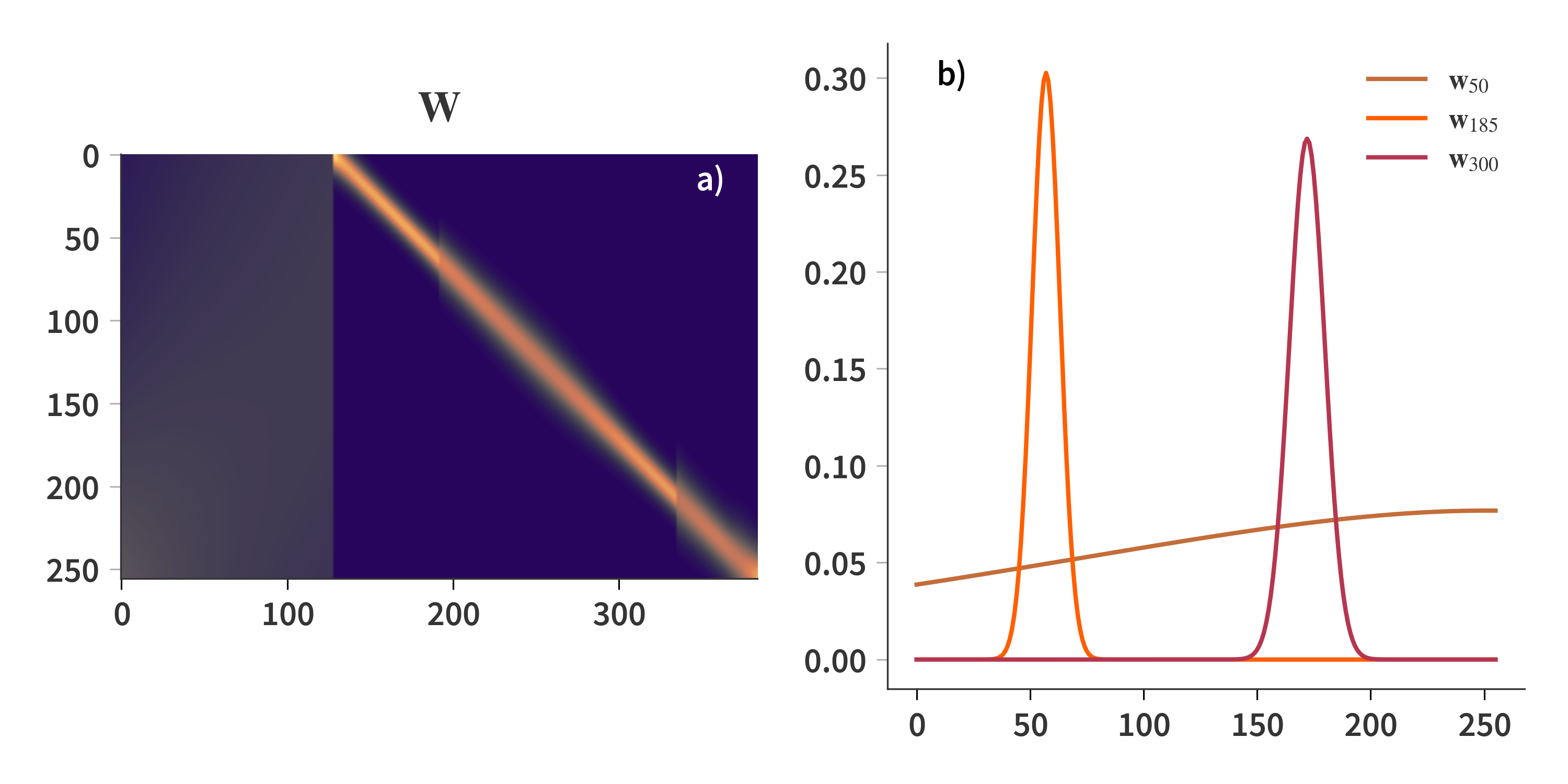
Let’s see how it works on the ground truth spectra. Here $\lambda = 10$
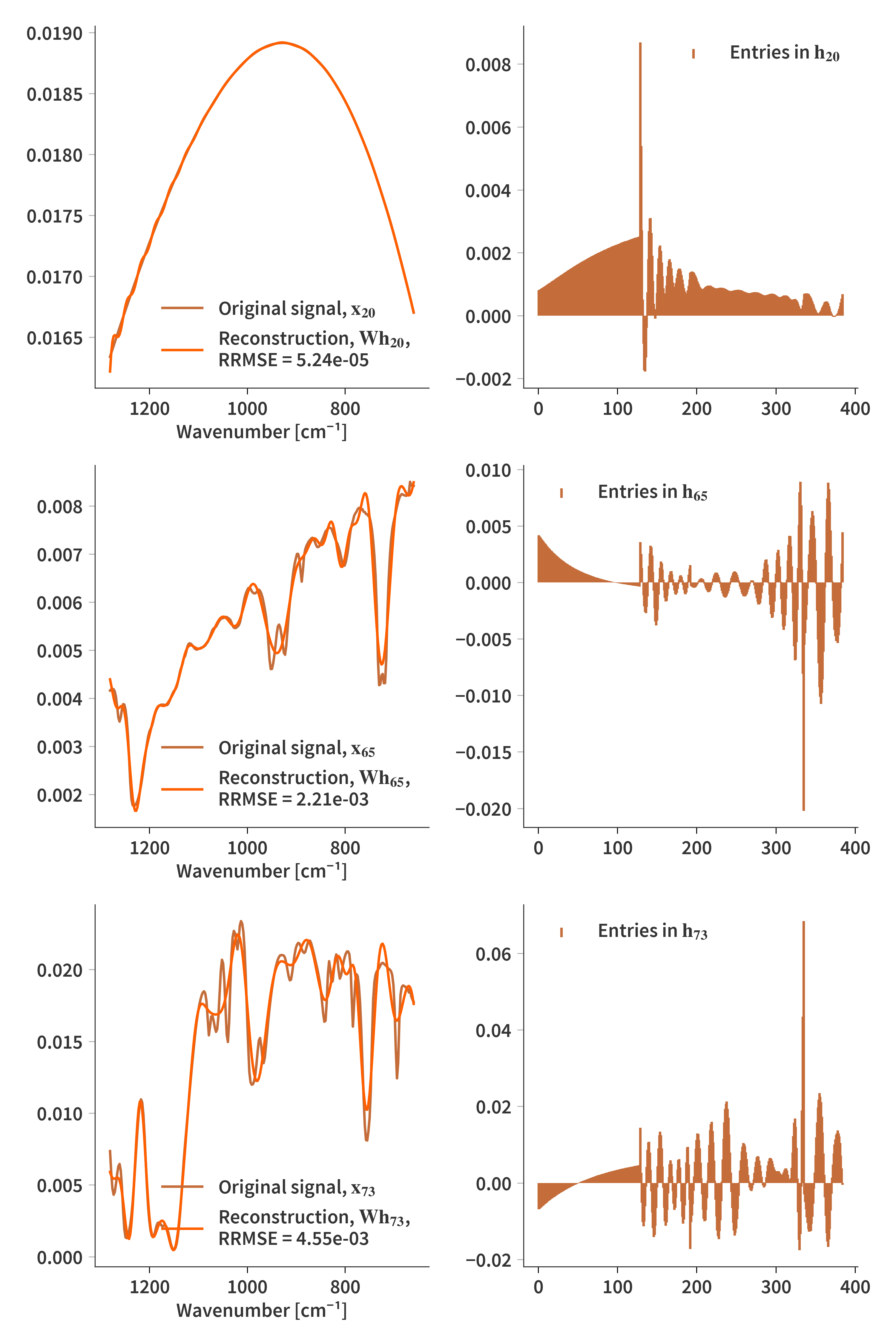
And then on reconstructions. Here $\lambda = 10^{-9}$
