Calculating frequency spectrum from interferograms
Updated:
This section will be mostly a selection of assorted notes on some of my findings as I have tried to convert from the mirror separation dependent interferograms to the frequency/wavelength dependent incident spectra. There will for this reason not be any real common thread going through the text.
Firstly, we must setup the model by calculating the total radiation flux both incident on the sensor but also the amount of flux leaving the system:
\[\begin{align} \label{eq:fpi_flux} \mathbf{\Phi} = \mathbf{T_{SFPI}}\diamond(\mathbf{t_{samp}}\circ\mathbf{m_{BB}}(T_{BB}) + (\mathbf{1} - \mathbf{t_{samp}})\circ\mathbf{m_{env}}(T_{env})) + \mathbf{R_{SFPI}} \diamond \mathbf{m_{sens}}(T_{sens}) \end{align}\]Here, $\circ$ and $\diamond$ represent element-wise (Hadamard product) and row/element-wise multiplication respectively. By row/element-wise I mean that each row of the matrix is multiplied element-wise by each element in the vector. $\mathbf{T_{SFPI}}$ and $\mathbf{R_{SFPI}}$ are the transmission and reflection matrices of the SFPI calculated using TMM. $\mathbf{t_{samp}}$ is the FTIR transmission spectrum of the sample. Since I do not have the reflectance spectra of the samples, these are estimated simply by $(\mathbf{1} - \mathbf{r_{samp}})$ (assuming the samples are loss-less). $\mathbf{m_{BB}}(T_{BB})$, $\mathbf{m_{env}}(T_{env})$, and $\mathbf{m_{sens}}(T_{sens})$ are the black body spectra of the black body behind the sample, the environmental background emission and the sensor. $T_{BB}$, $T_{env}$, and $T_{sens}$ are the temperatures of the black body, the environment, and the sensor respectively.
Since the signal measured by the microbolometer is related to the difference in $\mathbf{\Phi}$ and the flux of the sensor itself.
\[\begin{align} \label{eq:fpi_signal} \mathbf{\Delta\Phi} = \mathbf{\Phi} - \mathbf{m_{sens}}(T_{sens}) \end{align}\]Finally, the interferogram is related to the matrix-vector product of $\mathbf{\Delta\Phi}$ and the system response $\mathbf{s}$
\[\begin{align} \label{eq:sensor_response_Ax=b} \mathbf{i} = \mathbf{\Delta\Phi} \mathbf{s} \end{align}\]We know $\mathbf{i}$ (because we measured it), we have an estimate of $\mathbf{s}$ (from here) and we have a pretty good idea of some parts of $\mathbf{\Delta\Phi}$. The “unknown” part of $\mathbf{\Delta\Phi}$ is the spectrum of the subject:
\[\begin{align} \label{eq:unknown_part} \mathbf{x}=\mathbf{t_{samp}}\circ\mathbf{m_{BB}}(T_{BB}) + (\mathbf{1} - \mathbf{t_{samp}})\circ\mathbf{m_{env}}(T_{env}) \end{align}\]From here it is possible to rewrite and combine Eq. \ref{eq:fpi_signal}, \ref{eq:sensor_response_Ax=b} in order to transform the problem back into $\mathbf{Ax}=\mathbf{b}$. The right-hand-side becomes:
\[\begin{align} \label{eq:rhs} \mathbf{b}=\mathbf{i} - [\mathbf{R_{SFPI}} \diamond \mathbf{m_{sens}}(T_{sens}) - \mathbf{m_{sens}}(T_{sens})]\mathbf{s} \end{align}\]Note here that $\mathbf{m_{sens}}(T_{sens})$ is subtracted from each row in $\mathbf{R_{SFPI}} \diamond \mathbf{m_{sens}}(T_{sens})$ before the dotproduct of the entire thing and $\mathbf{s}$ is calculated. $\mathbf{A}$ then becomes:
\[\begin{align} \label{eq:A} \mathbf{A} = \mathbf{T_{SFPI}}\diamond\mathbf{s} \end{align}\]We are then left to find a method of calculating $\mathbf{x}$ from $\mathbf{A}$ and $\mathbf{b}$… and that turns out to be easier said than done…
Tikhonov regularization
The first attempt is calculating $\mathbf{x}$ directly from the pseudoinverse and tikhonov regularization. We define the regularization matrix $\mathbf{M}$ as
\[\begin{align} \label{eq:M_reg} \mathbf{M} = \begin{bmatrix} 1 & -1 & 0 & 0 & 0 & \dots \\ -1 & 2 & -1 & 0 & 0 & \dots\\ 0 & -1 & 2 & -1 & 0 & \dots\\ \vdots & \ddots & \ddots & \ddots & \ddots & \ddots\\ \dots & 0 & 0 & -1 & 2 & -1\\ \dots & 0 & 0 & 0 & -1 & 1\\ \end{bmatrix} \end{align}\]We can then solve for $\mathbf{x}$ directly
\[\begin{align} \label{eq:tikhonov_x} \mathbf{x} = (\mathbf{A}^T\mathbf{A} + \gamma \mathbf{M})^{-1}\mathbf{A}^T\mathbf{b} \end{align}\]Here, $\gamma$ is a regularization parameter controlling the influence of $\mathbf{M}$.
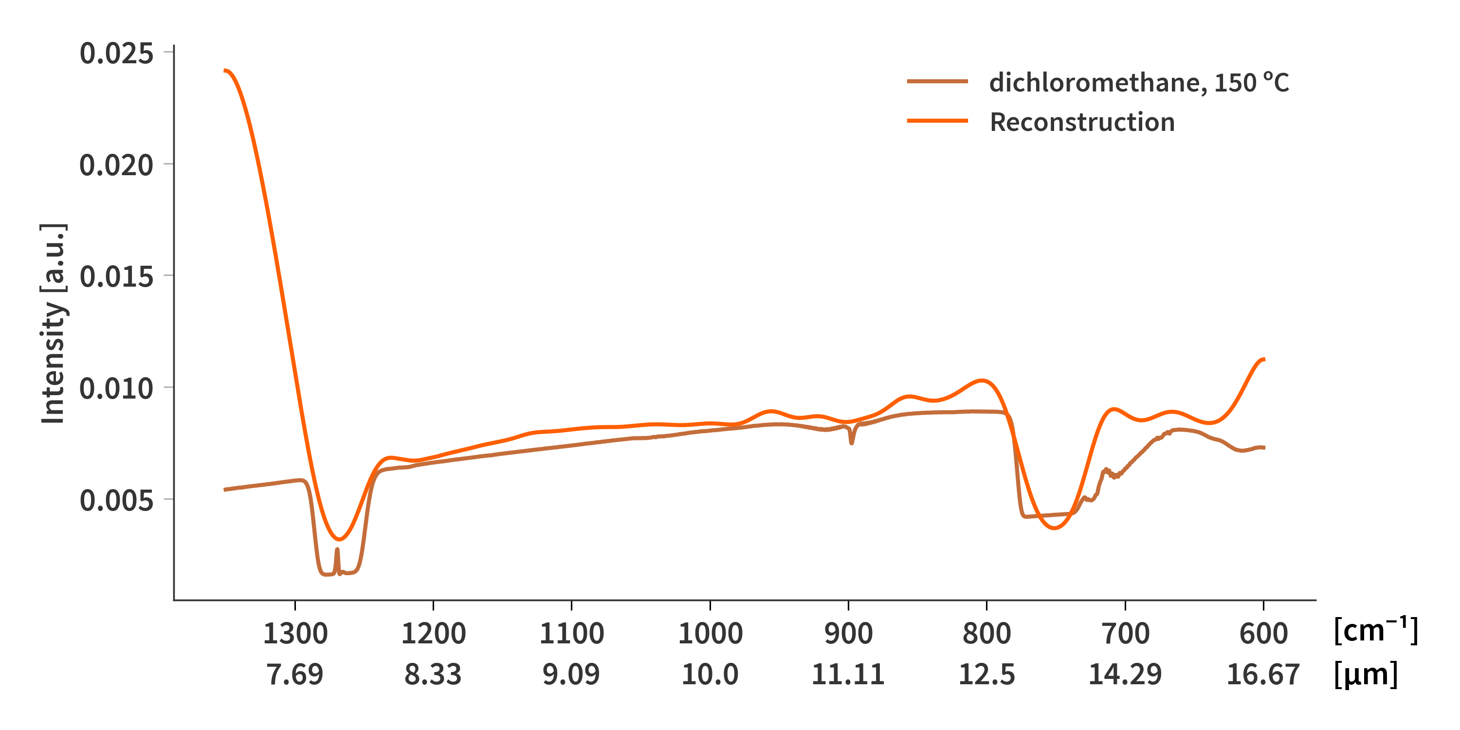
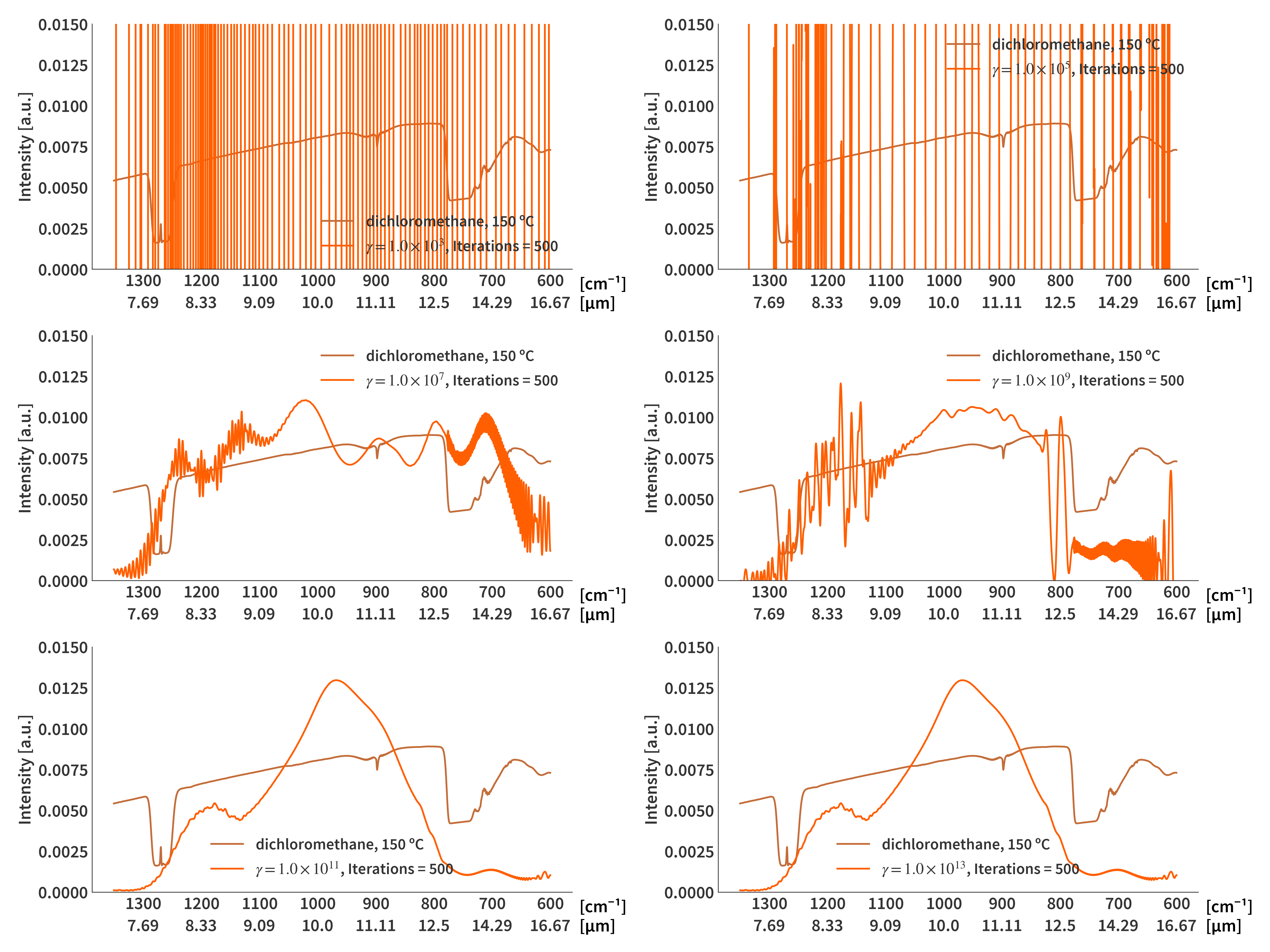
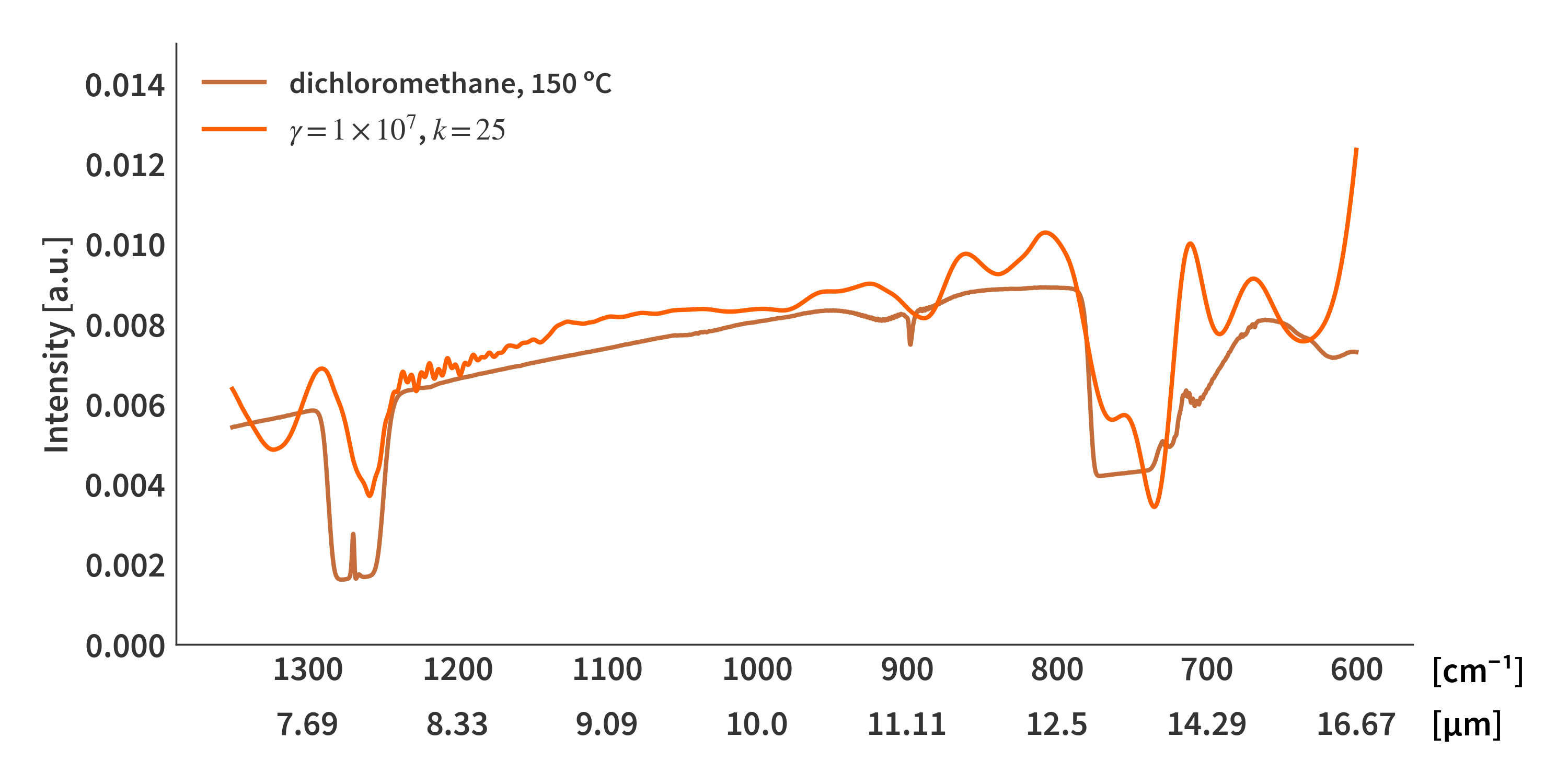
Trying to solve for the dichloromethane spectrum yields the result presented in Fig 1.
Gauss-Seidel
From “Iterative Methods for Sparse Linear Systems” by Yousef Saad.
This is an iterative row projection method.
\[\begin{align} \label{eq:gauss_seidel} &1. \quad\textrm{Choose initial } x\nonumber\\ &2. \quad\textrm{For }i = 1, 2, ..., n \textrm{ do}: \nonumber\\ &3. \quad\quad \delta_i = \omega \frac{b_i - \langle \mathbf{x} | \mathbf{A}^T\mathbf{e}_i \rangle}{‖\mathbf{A}^T\mathbf{e}_i‖_2^2} \nonumber\\ &4. \quad\quad \mathbf{x} = \mathbf{x} + \delta_i \mathbf{A}^T\mathbf{e}_i\nonumber \end{align}\]Here, $b_i$ represents the $i^\textrm{th}$ element of $\mathbf{b}$ and $\langle\mathbf{a}_1|\mathbf{a}_2\rangle$ is the inner dot product defined as $\mathbf{a}_1^\dagger\mathbf{a}_2$ with superscript $\dagger$ denoting the conjugate transpose. $\mathbf{e}_i$ is the $i^\textrm{th}$ column of the identity matrix which effectively means that $\mathbf{A}^T\mathbf{e}_i$ simply is the transpose of the $i^\textrm{th}$ row of $\mathbf{A}$. $\omega$ is denoted as a relaxation parameter.
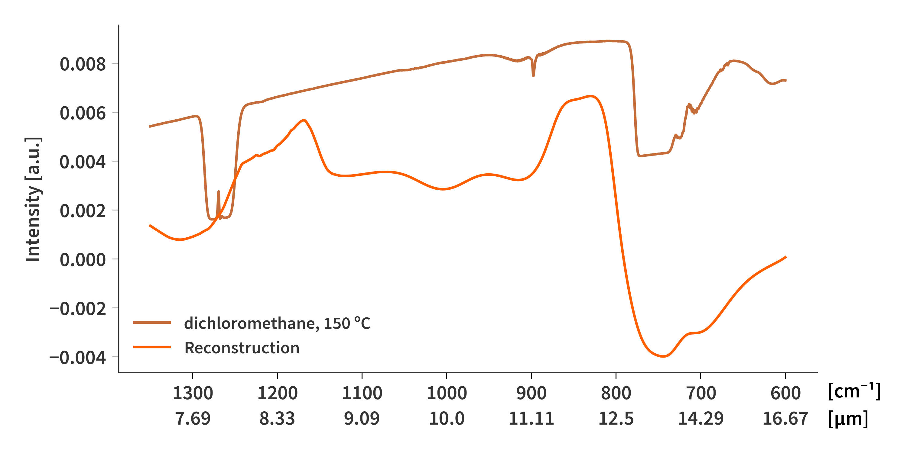
This method is relatively quick, but as seen in Fig. 2, not really that accurate. I also have not been able to implement Tikhonov regularization in this scheme - I am not quite sure why it does not work.
“Fast” Non-Negative Least Squares (FNNLS)
This least squares solver solves the $\mathbf{Ax}=\mathbf{b}$ problem subject to $\mathbf{x} >= 0$. The Tikhonov regularization is implemented the following:
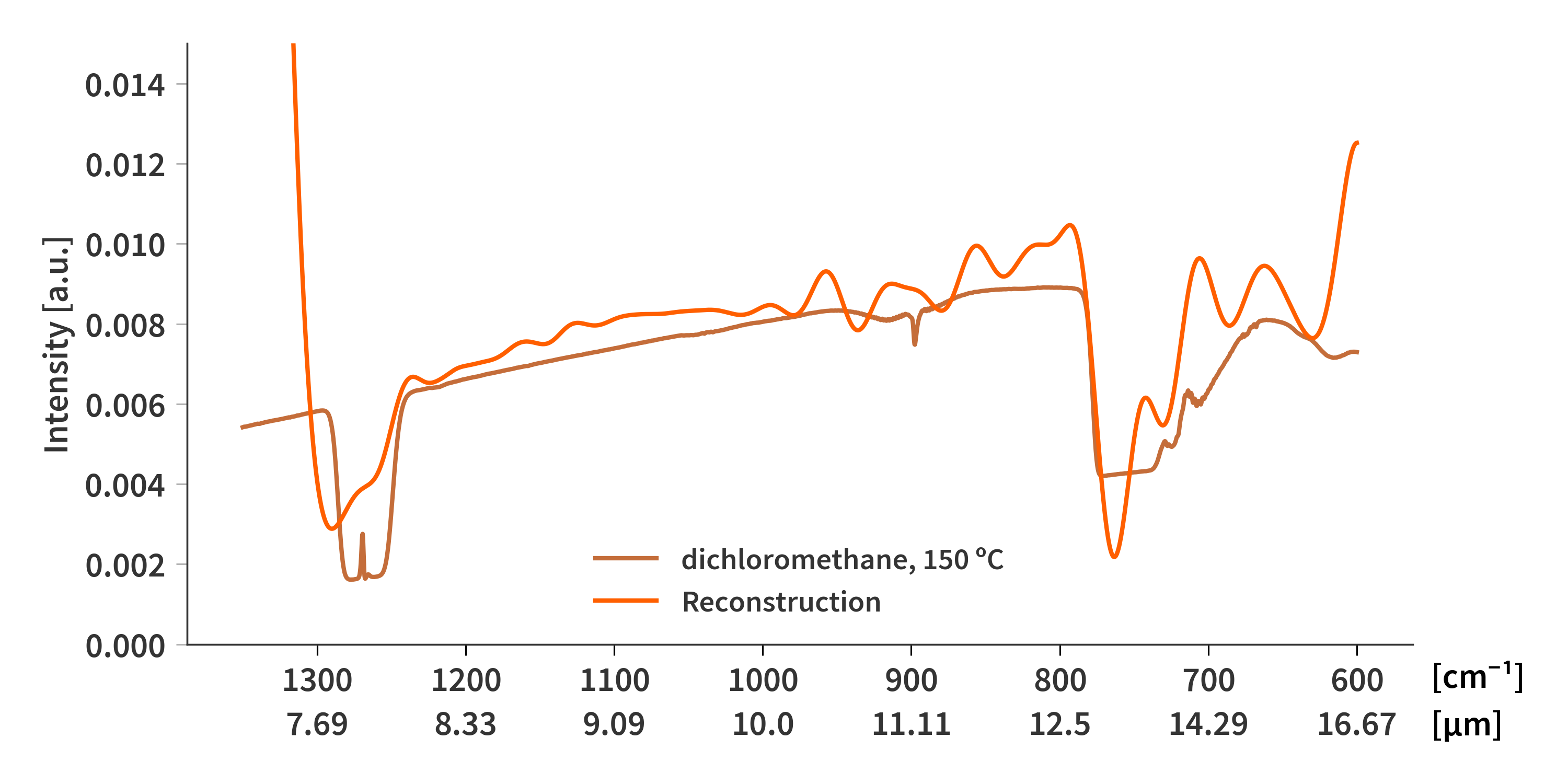
\[\begin{align} \label{eq:A_tilde} \mathbf{\tilde{A}} = \begin{bmatrix} \mathbf{A} \\ \gamma\mathbf{M} \end{bmatrix} \end{align}\] \[\begin{align} \label{eq:b_tilde} \mathbf{\tilde{b}} = \begin{bmatrix} \mathbf{b} \\ \mathbf{0} \end{bmatrix} \end{align}\]The FNNLS implementation in python is then used to solve $\mathbf{\tilde{A}x}=\mathbf{\tilde{b}}$. This however is VERY SLOW - upwards of 20 minutes on the M1 Macbook running full tilt. The result is shown in Fig. 3
Conjugate gradient (Craig’s method)
This one is also from “Iterative Methods for Sparse Linear Systems” by Yousef Saad. Here I have managed to do Tikhonov regularization in a similar way to the FNNLS method.
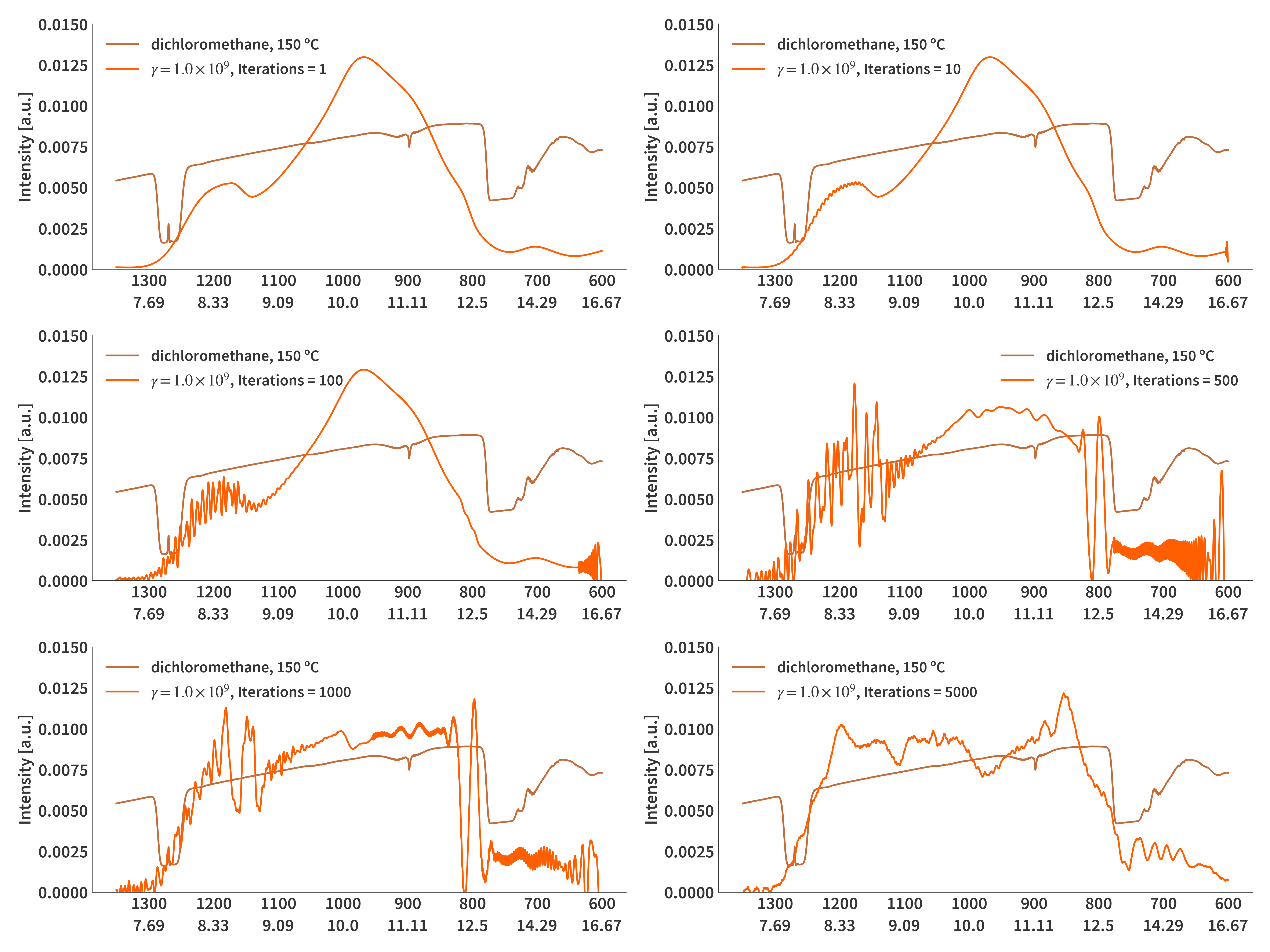
\[\begin{align} \label{eq:CGNE} 1.& \quad\textrm{Choose initial } x\nonumber\\ 2.& \quad \mathbf{r}_0 = \mathbf{\tilde{b}} - \mathbf{\tilde{A}x}_0 \nonumber\\ 3.& \quad \mathbf{p}_0 = \mathbf{\tilde{A}}^T\mathbf{r}_0 \nonumber\\ 4.& \quad\textrm{For }i = 1, 2, ... \textrm{ until convergence do}: \nonumber\\ 5.& \quad\quad \alpha_i = \langle\mathbf{r}_i | \mathbf{r}_i\rangle/\langle\mathbf{p}_i | \mathbf{p}_i\rangle \nonumber\\ 6.& \quad\quad \mathbf{x}_{i+1} = \mathbf{x}_i + \alpha_i \mathbf{p}_i\nonumber\\ 7.& \quad\quad \mathbf{r}_{i+1} = \mathbf{r}_i - \alpha_i \mathbf{\tilde{A}p}_i\nonumber\\ 8.& \quad\quad \beta_i = \langle\mathbf{r}_{i+1} | \mathbf{r}_{i+1}\rangle/\langle\mathbf{r}_{i} | \mathbf{r}_{i}\rangle \nonumber\\ 9.& \quad\quad \mathbf{p}_{i+1} = \mathbf{\tilde{A}}^T\mathbf{r}_{i+1} + \beta_i \mathbf{p}_i\nonumber\\ 10.&\quad\textrm{End do}\nonumber \end{align}\]For these calculations I have not set a convergence criterion but rather just an upper limit to the number of iterations. There are therefore two parameters to tweek the solver: The regularization parameter, $\gamma$ and the number of iterations - both of which have quite an impact on the solutions.
Of course the computation takes longer the more iterations are performed. 1000 iterations take around 15 seconds. Fig. 4 illustrate how the reconstructions are influenced by the number of iterations and Fig. 5 show how the regularization parameter affects the results.
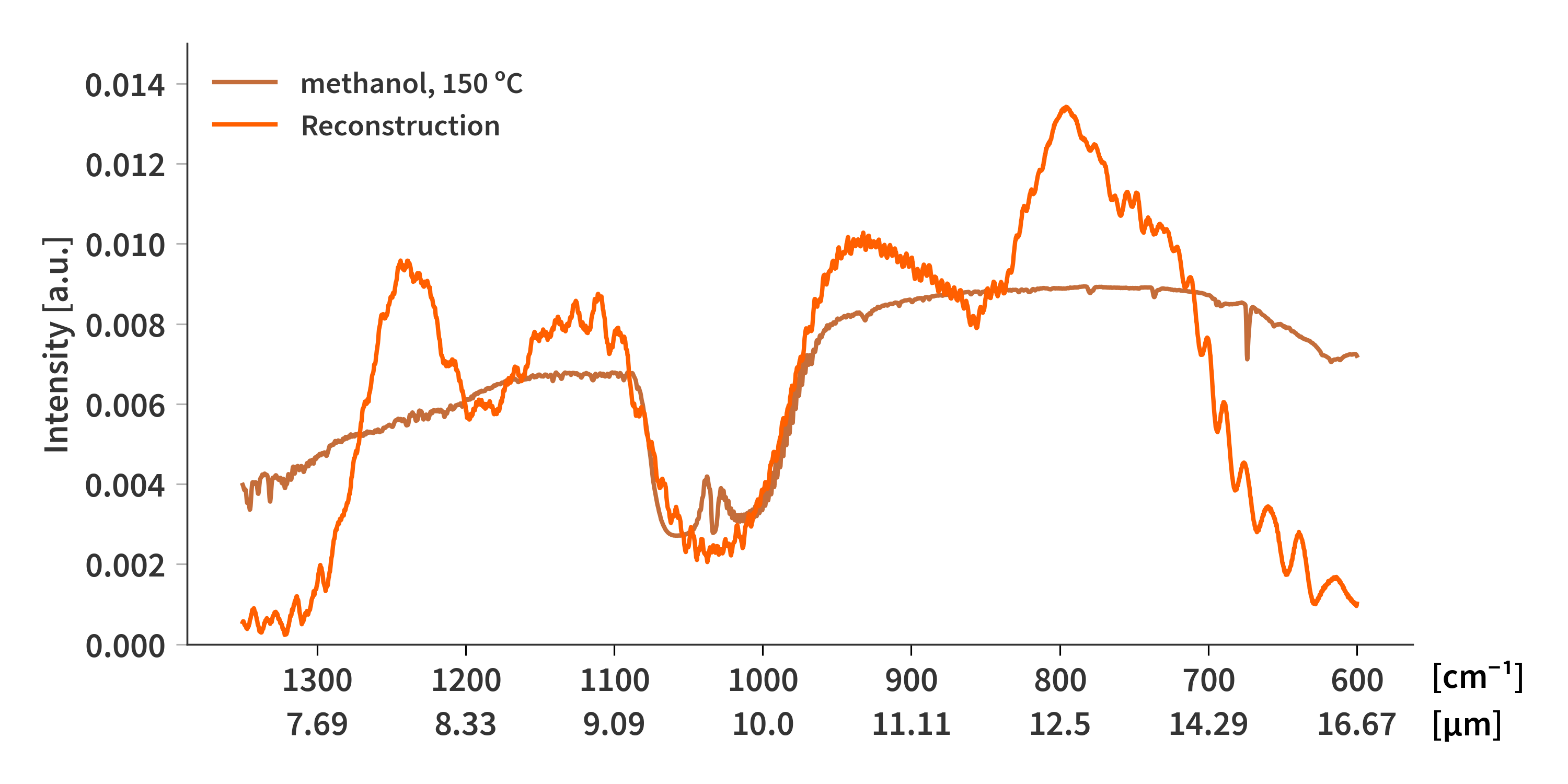
With the dichloromethane spectrum it might be a little difficult to judge whether the algorithm is doing anything at all since the two features are in either end of the spectrum, and the reconstructions tend towards zero at both ends. I tried using the same method on the methanol spectrum as presented in Fig. 6. Here It is clear to see that the method correctly captures the absorption bands at ≈ 9.5 µm. Still it is not a great fit.
Something about Krylov spaces?
The Krylov space is a subspace of $\mathbf{A}$ and $\mathbf{b}$:
\[\begin{align} \label{eq:krylov} \mathcal{K}_k = \textrm{span} \{\mathbf{A}^T\mathbf{b}, (\mathbf{A}^T\mathbf{A})\mathbf{A}^T\mathbf{b}, (\mathbf{A}^T\mathbf{A})^2\mathbf{A}^T\mathbf{b} \dots (\mathbf{A}^T\mathbf{A})^{k-1}\mathbf{A}^T\mathbf{b} \} \end{align}\]This forms a set of $k$ basis vectors which span $\mathcal{K}_k$ and they can even be orthonormal. An algorithm based on the Gram-Schmidt (QR-factorization) can be formulated (from chapter 6 in Discrete Inverse Problems: Insight and Algorithms.
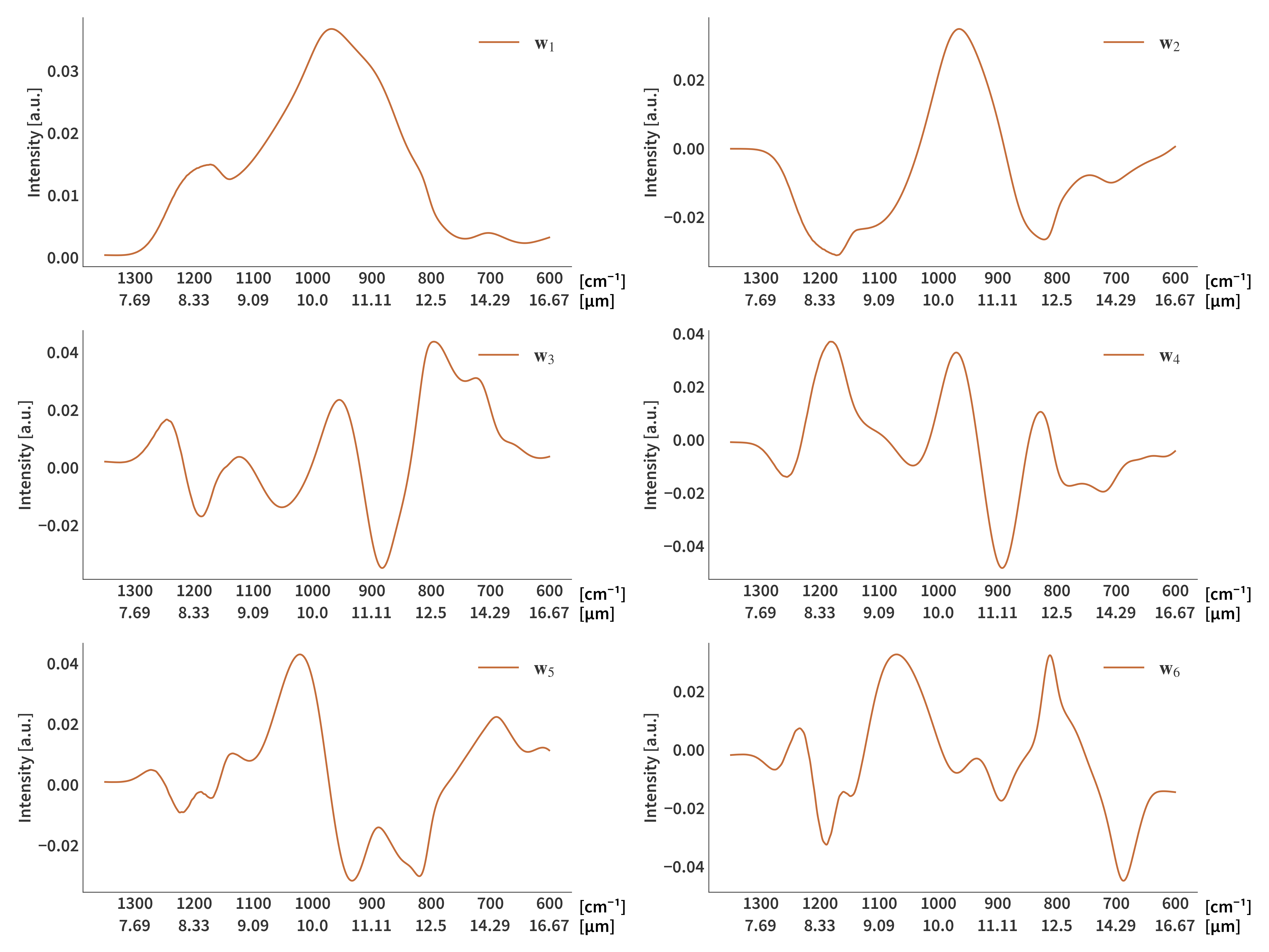
\[\begin{align} \label{eq:krylov_routine} 1.& \quad\textrm{Choose number of components, } k\nonumber\\ 2.& \quad \mathbf{w}_1 = \mathbf{A}^T\mathbf{b} \nonumber\\ 3.& \quad \mathbf{w}_1 = \mathbf{w}_1 / ‖\mathbf{w}_1‖_2 \nonumber\\ 4.& \quad\textrm{For }i = 2, 3, ... k \textrm{ do}: \nonumber\\ 5.& \quad\quad \mathbf{w}_i = \mathbf{A}^T\mathbf{A}\mathbf{w}_{i-1} \nonumber\\ 6.& \quad\quad \textrm{For }j = 1, ... i-1 \textrm{ do}: \nonumber\\ 7.& \quad\quad\quad \mathbf{w}_i = \mathbf{w}_i - (\mathbf{w}_j^T\mathbf{w}_i)\mathbf{w}_j\nonumber\\ 8.& \quad\quad \mathbf{w}_i = \mathbf{w}_i / ‖\mathbf{w}_i‖_2 \nonumber\\ \end{align}\]Each vector $\mathbf{w}_i$ form the columns of the matrix $\mathbf{W}$. The higher the component, the higher the frequencies are represented in the signal (Fig. 7).
It is then possible to use $\mathbf{W}$ as basis vectors and project $\mathbf{Ax} = \mathbf{b}$ onto them by setting:
\[\begin{align} \label{eq:krylov_Ax_b} &\mathbf{x}^{(k)} = \mathbf{W}_k \mathbf{y}^{(k)} \\ \Rightarrow & \mathbf{y}^{(k)} = \textrm{argmin}_y ‖\mathbf{AW}_k\mathbf{y} - \mathbf{b}‖_2 \end{align}\]which can then be solved for $\mathbf{y}$ in any way we as we see fit. Firstly, I will solve it naively by simply using:
\[\begin{align} \label{eq:solve_krylov} &\mathbf{A'}_{k} = \mathbf{AW}_k \\ & \mathbf{y}^{(k)} = (\mathbf{A'}_k^T\mathbf{A'}_k)^{-1}\mathbf{A'}_k^T\mathbf{b} \end{align}\]Fig 8 illustrates how $k$ influences the solutions. The more components are included in the projection, the more unstable/noisy the solution.
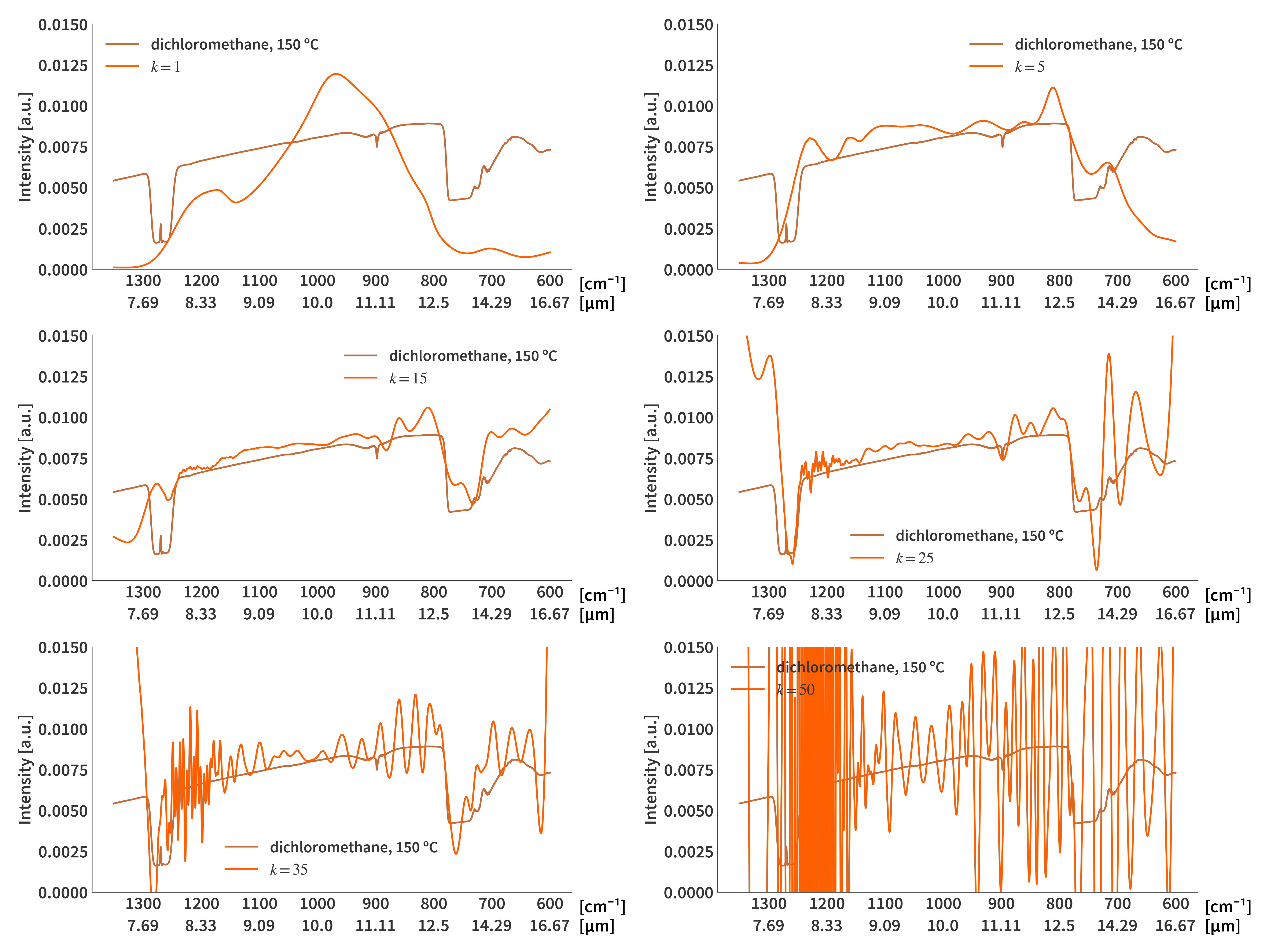
We can then use Tikhonov regularization as usual when solving for $\mathbf{y}^{(k)}$. This has the expected effect off lowering the amount of oscillations as depicted in Fig. 9.
Nonnegative matrix factorization
The idea is similar to what has just been shown in the section about Krylov spaces, but here we are going to introduce a couple of additional constraints. We are going to factorize the original spectra into a linear combination of atoms. We are essentially constructing a dictionary of possible solutions. That means that when reconstructing a spectrum from an interferogram, instead of having infinitely many possible solutions, we require the solution to be some combination of the “solutions” in the dictionary. We train a model to only propose more or less physical spectra when solving. For this part we don’t need interferograms to compare against nor do we need a perfect system matrix - we are just looking for possible solutions to the reconstruction problem. Therefore, the more spectra the better - but firstly, we are only going to consider the relevant ones from these experiments.
We are out to find an algorithm which can calculate a dictionary, $\mathbf{W}$, which fit the training data, and a coefficient matrix, $\mathbf{H}$ which is used to combine the atoms of the dictionary to best match the original signal. The spectra are kept in the columns of the matrix $\mathbf{X}$ and is factorized following.
\[\begin{align} \label{eq:NMF} \mathbf{X} \approx \mathbf{WH}, \qquad \mathbf{X} \in \mathbb{R}^{M \times N}, \qquad \mathbf{W} \in \mathbb{R}^{M \times R}, \qquad \mathbf{H} \in \mathbb{R}^{R \times N} \end{align}\]We want the atoms to all be positive as negative spectra does note really make sense. Similarly, the coefficients i $\mathbf{H}$ should also all be positive. We can therefore set up the following minimization problem.
\[\begin{align} \label{eq:arg_min} \arg \min_{\mathbf{W,H}} ||\mathbf{X} - \mathbf{WH}||_F^2 + \lambda||\mathbf{MW}||_F^2 + \gamma||\mathbf{H}||_\textrm{1, columns} \qquad \textrm{s.t.} \quad \mathbf{W,H} \geq 0 \end{align}\]where the additional regularization term $||\mathbf{MW}||_F^2$ has been added to smooth the atoms of $\mathbf{W}$, as they otherwise become very noisy. $\mathbf{M}$ is therefore an $M \times M$ matrix similar to what is shown in Eq. (\ref{eq:M_reg}). Furthermore, we want the columns of $\mathbf{H}$ to be sparse which is encuraged by the $||\mathbf{H}||_\textrm{1, columns}$ regularization term.
We are going to minimize the cost function using a gradient decent algorithm. This requires us to take the partial derivative of Eq. (\ref{eq:arg_min}) with respect to both $\mathbf{W}$ and $\mathbf{H}$ separately. A more thorough derivation can be seen here, but it essentially boils down to this:
The update functions are defined as:
\[\begin{align} \label{eq:W_update} \mathbf{W} &\leftarrow \mathbf{W} - \alpha_\mathbf{W}\nabla_\mathbf{W} f(\mathbf{W,H}) \\[1.2em] \mathbf{H} &\leftarrow \mathbf{H} - \alpha_\mathbf{H}\nabla_\mathbf{H} f(\mathbf{W,H})\label{eq:H_update} \end{align}\]where $\alpha_\mathbf{W}$ and $\alpha_\mathbf{H}$ are step sizes and $f(\mathbf{W,H})$ is the cost function defined as:
\[\begin{align} \label{eq:cost_function} f(\mathbf{W,H}) = ||\mathbf{X} - \mathbf{WH}||_F^2 + \lambda||\mathbf{MW}||_F^2 + \gamma||\mathbf{H}||_\textrm{1, columns} \end{align}\]Calculating the gradient of $f(\mathbf{W,H})$ w.r.t. both $\mathbf{W}$ and $\mathbf{H}$ leads to the update functions being:
\[\begin{align} \label{eq:W_update2} \mathbf{W} &\leftarrow \mathbf{W} - \alpha_\mathbf{W}(\mathbf{WWH}^T - \mathbf{XH}^T + \lambda\mathbf{M}^T\mathbf{MW}) \\[1.2em] \mathbf{h} &\leftarrow \mathbf{h} - \alpha_\mathbf{h}(\mathbf{W}^T\mathbf{Wh} - \mathbf{W}^T\mathbf{x} - \gamma\mathbf{1})\label{eq:H_update2} \end{align}\]The update function for $\mathbf{H}$ only operates on a single column $(\mathbf{h})$ at a time, while the update function for $\mathbf{W}$ updates the entire matrix at once. As for the step sizes, then theory predicts that the step sizes should lie in the interval $0 \leq \alpha \leq \frac{2}{L}$ where $L$ is the Lipschitz constant. From this it follows that
\[\begin{align} \label{eq:stepsize_W} 0\leq \alpha_\mathbf{W} & \leq \frac{1}{||\mathbf{\mathbf{HH}^T}||_2 + \lambda||\mathbf{\mathbf{M}^T\mathbf{M}}||_2} = \frac{1}{\sigma_1(\mathbf{H}) + \lambda \sigma_1(\mathbf{M})} \\[1.2em] 0\leq \alpha_\mathbf{h} & \leq \frac{1}{||\mathbf{\mathbf{W}^T\mathbf{W}}||_2} = \frac{1}{\sigma_1(\mathbf{W})} \label{eq:stepsize_H} \end{align}\]where $\sigma_1(\mathbf{A})$ is the largest singular value of the matrix $\mathbf{A}$. The singular values are related to the eigenvalue following $\sigma_i^2 = \lambda_i$ following $\sigma_i^2(\mathbf{A}) = \lambda_i(\mathbf{A}^*\mathbf{A})$. Caution, here $\lambda_i$ refers to the $i^\textrm{th}$ eigenvalue and NOT the regularization parameter.
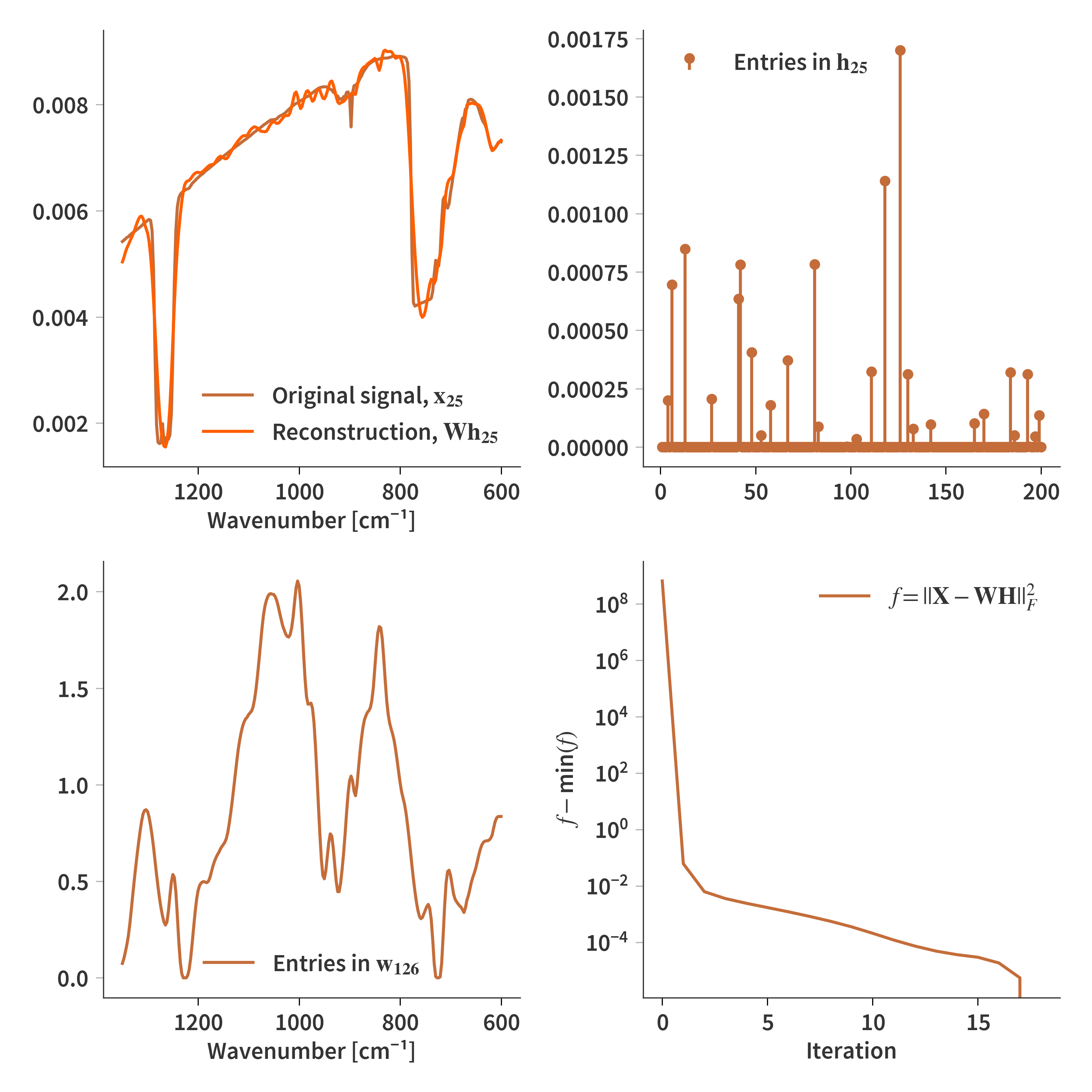
$\mathbf{W}$ and $\mathbf{H}$ are initialized as random numbers between 0 and 1, after which the update functions are run multiple times (in this case 18). The regularization parameters are $\gamma = 1\times10^{-2}$ and $\lambda = 1\times10^{-3}$ while the step sizes are set to $1/L$ (not $2/L$).
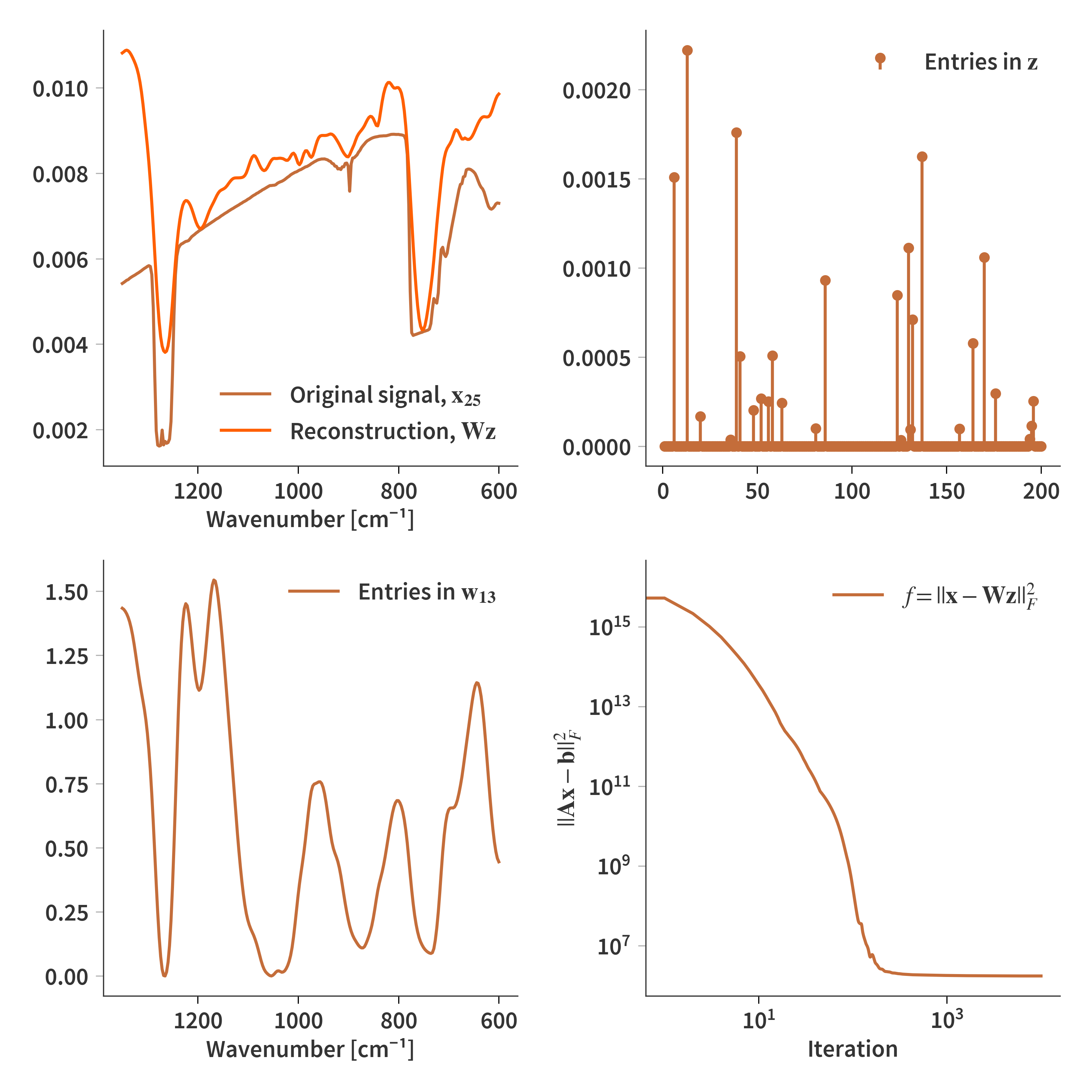
That was only the first part of the problem. We still need to reconstruct one of the interferograms - that is, solve $\mathbf{Ax} = \mathbf{b}$. $\mathbf{A}$ is still the system matrix and $\mathbf{b}$ is the corrected interferogram as in Eq. (\ref{eq:rhs}). However, we want to solve the problem in terms of the sparse basis. That means that the minimization problem can be reformulated
\[\begin{align} \label{eq:arg_min_sparse} &\arg \min_{\mathbf{x}} ||\mathbf{b} - \mathbf{Ax}||_F^2 \\[1.2em] &\arg \min_{\mathbf{z}} ||\mathbf{b} - \mathbf{ADz}||_F^2 + \gamma||\mathbf{z}||_1 \\[1.2em] \end{align}\]This allows us to use the same update function as presented in Eq. (\ref{eq:H_update2}) to calculate the sparse solution $\mathbf{z}$. The original spectrum can then be recovered by $\mathbf{Dz}$. The final reconstruction can be seen in Fig. 11 below.
An argument to describe the incident spectrum with negative terms (only relevant for spectral reconstruction)
Even though light intensity cannot be negative, I could make the argument that the emission spectrum of any given object in a scene can be treated as a perfect black-body emitter at a given temperature. The deviations from a perfect black-body are then determined by its emissivity (which is a spectral property). The emissivity $\varepsilon(\lambda)$ is a number between 0 and 1 and changes with the wavelength:
\[\begin{align} \label{eq:emissivity} \varepsilon(\lambda) = \frac{M_{obj}(T, \lambda)}{M_{BB}(T, \lambda)} \end{align}\]The signal can still not become negative, but if the black-body is the “baseline”, then “subsignals” can be subtracted until the true spectrum is recovered. This way the proposed solution should never overshoot the black body eliminating non-physical solutions from the space of possible solutions.
