Hyperspectral image viewer
I have made a hyperspectral image viewer/analyser has been programmed in python utilizing the Tkinter library. The program makes it possible to do some simple data processing as well as extracting mean spectra based on user definable colored selections.
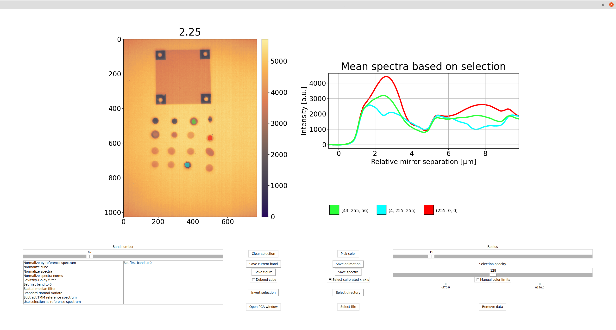
Here is an example of a hyperspectral thermal image of a collection of different gemstones being displayed in the viewer.

Basic operations
Loading an image
If the image comes out of the hyperspectral thermal camera, it is loaded using the Select directory button. Here, the directory containing the “/images/capture/” (this matches the standard data output of the camera) must be located. If the hyperspectral image is instead in “.pam” or “.npy” format, choose the Select file button instead. The numpy array must have exactly three dimensions where axis 2 (the third dimension) contains the spectral information.
Scrolling through the bands
Using the leftmost slider with Band number written above it, it is possible to scrub through the bands of the data cube. While moving the slider, the image of the viewer is updated. By default, the color range changes with every new band, but it is possible to fix the range by checking the Manual color limits check box in the bottom right corner. The accompanying slider can then be used set the lower and upper limits of the color range.
Extracting mean spectrum/interferograms
It is possible to use the mouse to draw a selection directly on the image on the right. By left clicking and dragging the mouse, a colored mask is drawn and shown on top of the image. Once the mouse button is released, the mean spectrum is plotted in the corresponding color in the plot on the right. The size of the brush (measured in pixels) can be changed with the slider, Radius, and the opacity of the mask can be changed with the Selection opacity slider. Right clicking on the image can be used to erase existing color mask, and the Clear selection button can be used to clear all selections at once and the Invert selection button converts all selections to the same color after which the mask is inverted. Different colors can be selected using the Pick color button. Once a color has been added to the mask, it will appear as a color swatch under the plot on the right. By clicking a swatch, the associated color is ‘brought to the front’ and is made active again - making it possible to add to the mask without having to enter the exact same RGB value again.
Calibrated x-axis
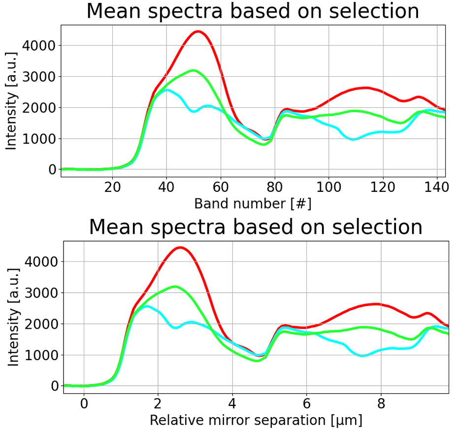
By default, the x-axis of the data cube is simply a list of integers corresponding to the number of channels in the cube. By checking the Select calibrated x axis check box, the user is presented with a number of options as presented in the screen shot below.

The first two options are proprietary for the hyperspectral thermal camera. The Relative mirror separation option is the easiest as this automatically calculates how far the mirrors have moved based on the interferograms of the three laser diodes, which are used to maintain smooth and consistent movement of the mirrors. If this option is chosen, the user is prompted to enter a offset value. This offset value is often not known, and an offset of 0.0 µm is used instead. From the screenshot below it is evident that the mirrors have not moved an equal distance between each channel of the data cube.

The Numpy polynomial (.npy) option is a legacy options from when a third order polynomial is used to generate the x-axis based on the number of spectral channels. By clicking this option, a file explore is opened, and the polynomial coefficients saved as a .npy file can be selected.
The final option is Vector (.npy, .txt, or .csv). His allows the user to chose their own x-axis saved in one of the aforementioned formats. The vector must of cause have the same number of entries as the number of spectral channels in the cube.
The Select x-axis dialog box is also summoned by other preprocessing steps if selected with the standard linear x-axes. These are only relevant for data coming from the hyperspectral thermal camera.
Removing data
It is possible to remove entire sections of a data cube based on a selection. Simply paint the parts of the image you would like to exclude from the analysis, then hit the Remove data button, and the data will be replaced by NaNs, effectively excluding them from the preprocessing.
Saving files
It is possible to save different forms of images using the viewer. The Save current band button saves the current band in the viewer as a 8-bit .tif file. Save figure saves the entire figure (both image, plot and color swatches) as a .png. Save animation saves the data cube as a .gif with 10 FPS. The Save spectra button saves all extracted spectra either as a .txt (default) or .csv file. The first column of the file contains the x-axis. The following columns are arranged from most recent to oldest markings on the color mask. This means that column 1 (0-indexing for the x-axis) is bottom leftmost color swatch, column 2 corresponds to the color swatch to its right and so on.
At this moment it is not possible to save preprocessing steps or color masks applied in the viewer.
Adding preprocessing and data analysis
The hyperspectral image viewer makes it possible to apply different forms of preprocessing to the entire image. Preprocessing steps labeled with (Only HSTC) can only be applied to data coming from the hyperspectral thermal camera. In the following, $\mathbf{s}(x,y)$ refers to the spectrum found in the pixel located at $(x,y)$ and is a vector. $\mathbf{S_\lambda}$ refers to a specific spectral channel and is a matrix. E.g., $\mathbf{S_0}$ refers to the first spectral channel. $s_5(x,y)$ refers to the pixel at location $(x,y)$ in the fifth spectral channel- this is a scalar. If neither subscript $\lambda$ nor coordinates $(x,y)$ are given, then $\mathbf{S}$ refers to the entire data cube at once.
Apply NUC (Only HSTC)
Autoscale
The autoscale function is used to center and scale each spectral channel in the data cube. Firstly, each channel is mean centered after which it is scaled by its standard deviation.
\begin{equation} \label{eq:autoscale}
\mathbf{S}_{\lambda, new} = \frac{\mathbf{S}_\lambda - \bar{\mathbf{S}}_{\lambda}}{\sigma_{\mathbf{S}_\lambda}},
\end{equation}
where $\bar{\mathbf{S}}_{\lambda}$ and $\sigma_{\mathbf{S}_\lambda}$ are the mean and standard deviation of the $\lambda^\textrm{th}$ channel respectively.
Convert to wavelength (Only HSTC)
Debend cube (Only HSTC)
Correct laser spot (Only HSTC)
This function is used to remove some pixels affected by exposure to a 10.6 µm laser as described here. In this case 30 pixels are replaced by a linear interpolation based on their closest neigbourhood - 10×10 pixels including the affected 30 pixels). This is done for each channel in the data cube.
Correct laser spot LARGE (Only HSTC)
Same as the one above, but instead of just 30 pixels, a 16×16 pixel region is selected. The two outermost rows/columns are used to interpolate the values of the central 14×14 pixels.
Mean center bands
As the name suggests, this function takes each spectral channel and subtracts its mean.
\begin{align} \label{eq:mean_center_bands}
\mathbf{S}_{\lambda, new} = \mathbf{S}_\lambda - \bar{\mathbf{S}}_\lambda
\end{align}
Mean center spectra
Similarly, this function subtracts the mean of each spectrum.
\begin{align} \label{eq:mean_center_spec}
\mathbf{s}_{new}(x,y) = \mathbf{s}(x,y) - \bar{\mathbf{s}}(x,y)
\end{align}
Normalize band norms
This function divides each spectral channel by its norm.
\begin{align} \label{eq:norm_band_norms}
\mathbf{S}_{\lambda, new} = \frac{\mathbf{S}_\lambda}{|\mathbf{S}_\lambda|},
\end{align}
Normalize by reference spectrum (Only HSTC)
Normalize cube
This function takes the entire cube and offsets it and scales it to span from a minimum value of 0 to a maximum value of 1.
\begin{align} \label{eq:normalize_cube_offset}
\mathbf{S}_{offset} = \mathbf{S} - \textrm{min}\left(\mathbf{S}\right),
\end{align}
\begin{align} \label{eq:normalize_cube}
\mathbf{S}_{new} = \frac{\mathbf{S}_{offset}}{\textrm{max}\left(\mathbf{S}_{offset}\right)},
\end{align}
Normalize spectra
This function scales each individual spectrum in the data cube to span from a minimum of 0 to a maximum of 1.
\begin{align} \label{eq:norm_specs_offset}
\mathbf{s}_{offset}(x,y) = \mathbf{s}(x,y) - \textrm{min}\left(\mathbf{s}(x,y)\right),
\end{align}
\begin{align} \label{eq:norm_specs}
\mathbf{s}_{new}(x,y) = \frac{\mathbf{s}_{offset}(x,y)}{\textrm{max}\left(\mathbf{s}_{offset}(x,y)\right)},
\end{align}
Normalize spectra norms
This function divides each spectrum in the data cube by its norm.
\begin{align} \label{eq:norm_spec_norms}
\mathbf{s}_{new}(x,y) = \frac{\mathbf{s}(x,y)}{|\mathbf{s}(x,y)|},
\end{align}
Savitzky-Golay filter
This function is a simple implementation of the Scipy savgol_filter() function. The user is prompted to enter the number of samples, the polynomial order as well as the derivative degree of the filter which is then applied to the spectral axis.
Set first band to 0
The first spectral channel is subtracted from each layer of the cube. For a single layer this looks like: \begin{align} \label{eq:set_first_2_0} \mathbf{S}_{\lambda, new} = \mathbf{S}_\lambda - \mathbf{S}_0 \end{align} This is repeated for all spectral channels.
Spatial median filter
This is an implementation of the Scipy median_filter() function. The user is prompted to input a kernel size, which must be an odd integer. Afterwards, this filter is applied to each spectral channel of the data cube.
Standard Normal Variate
Also sometimes referred to by its abbreviation, SNV. This step is used to minimize differences between pixels due to intensity variations such that spectral differences are enhanced.
\begin{align} \label{eq:SNV}
\mathbf{s}_{new}(x,y) = \frac{\mathbf{s}(x,y) - \bar{\mathbf{s}}(x,y)}{\sigma_{\mathbf{s}(x,y)}},
\end{align}
where $\bar{\mathbf{s}}(x,y)$ and $\sigma_{\mathbf{s}(x,y)}$ are the mean and standard deviation of the spectrum in pixel $(x,y)$ respectively.
Subtract TMM reference spectrum (Only HSTC)
Use selection as reference spectrum
This function takes the mean of the most recent selection and compares the rest of the data cube to this spectrum. This implies that the difference between this reference and every other spectrum is calculated as follows.
\begin{align} \label{eq:reference_spec_selection} \mathbf{s}_{new}(x,y) = \bar{\mathbf{s}}_{selection} - \mathbf{s}(x,y) \end{align}
Principal Component Analysis
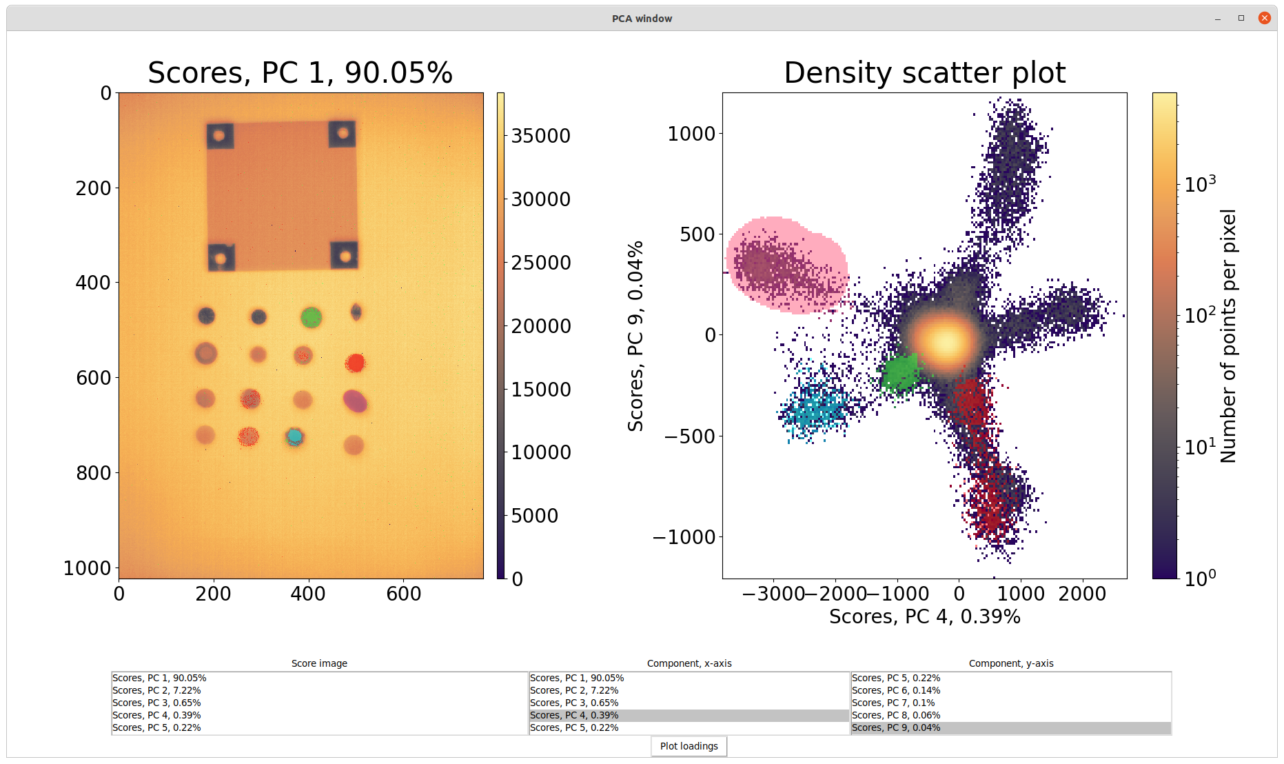
The principal components (PCs) of the data cube is calculated and presented in a new window by pressing the Open PCA window button. On the left of the screen are the score image presented for all PCs one a a time. Scores of different PCs can be selected from the list below the image. On the right is a density scatter plot showing a 2D slice of the PCA space. What dimensions the data is projected onto can be chosen from the two lists Component, x-axis and Component, y-axis below the plot. The colorbar indicate how many pixels are binned in the same pixel of the plot. The percentages shown along with each PC indicate how much of the total variance is explained by this single component.
It is possible to color in different parts of the score image and see where in the PC space these show up. Whatever is the foreground color and brush radius of the main window of the Hyperspectral viewer is also the brush settings for the PCA window. Hereby it is possible to color in the same stones as the extracted spectra from the viewer and see how they are separated in different PCs. Likewise it is also possible to color in the density scatter plot and find out which pixels correspond to each cluster. In the image below, a pink color have been used to select the upper left most branch of the density scatter plot. It can hereby be concluded that the gem stone in the last column and second to last row is responsible for this cluster.

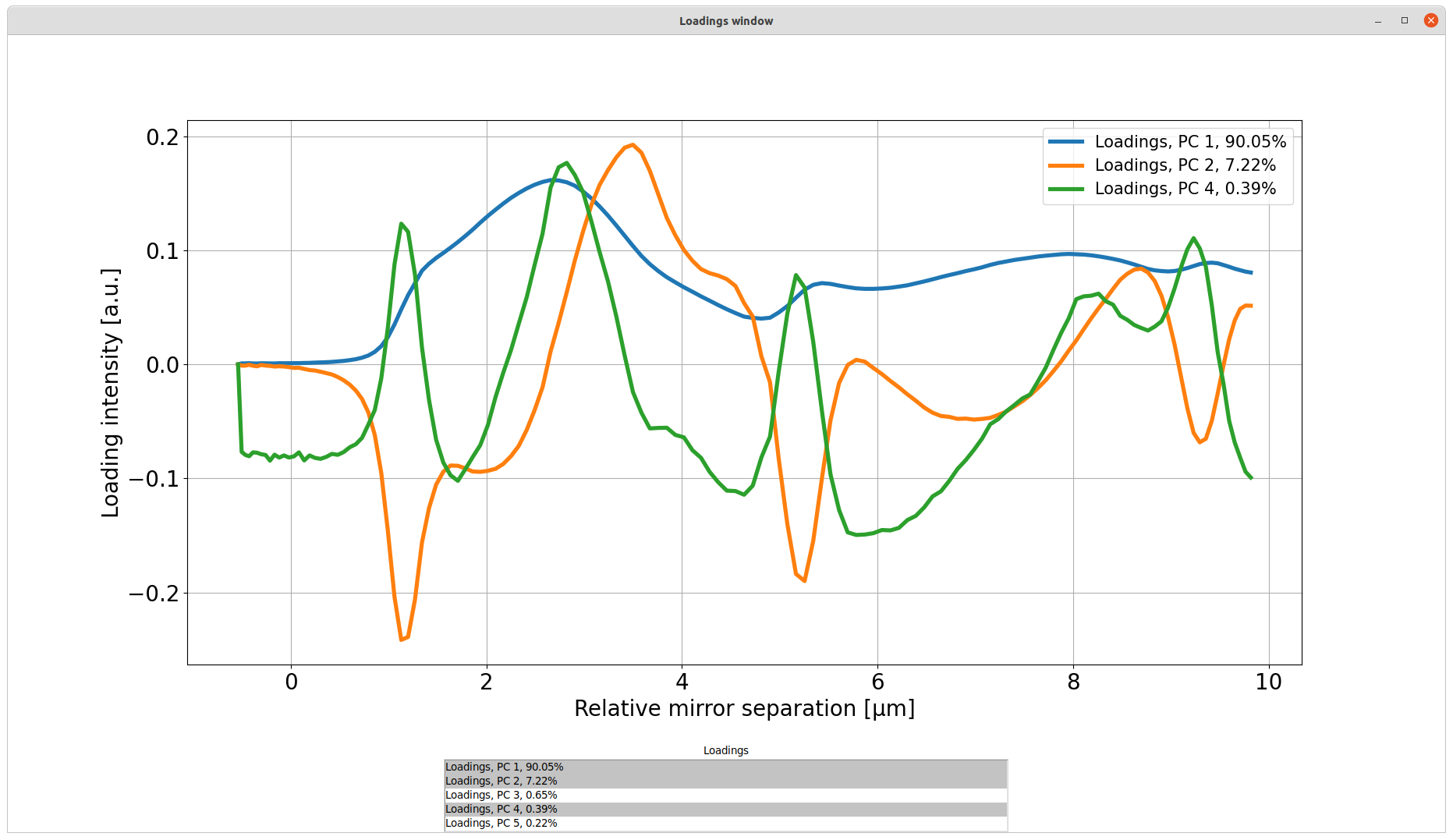
By pressing the Plot loadings button, a new window appears. Here it is possible to plot the loadings of each PC on top of each other for comparison. Multiple components can be selected from the list at the same time. To deselect a PC, simply click it again.

